Cumulative Spectral Decay Plots
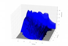
As an educational exercise I wrote a short python script which makes CSD plots from the impulse responses exported by HOLM Impulse. From the experience I am surprised by what the plots can reveal or hide to the viewer with different amplitude and time axis parameters. I think I will definitely be a more skeptical in assessing waterfall plots. The code is provided below if anyone would like to play with it.
As an educational exercise I wrote a short python script which makes CSD plots from the impulse responses exported by HOLM Impulse. From the experience I am surprised by what the plots can reveal or hide to the viewer with different amplitude and time axis parameters. I think I will definitely be a more skeptical in assessing waterfall plots. The code is provided below if anyone would like to play with it.
Code:
# Author: Roger Lew
# Date: 7-15-2010
# Version: .1
# Copyright: Public Domain, do what you want with it

"""
This script creates csd plots from ASCII text impulse response files. The impulse
response file should begin at time 0 and have a power of 2 number of samples
the file should have only one column with the amplitude values by time. The sampling
rate (as well as other parameters for the plot) should be specified below. The script
should open a window which will allow you to manually rotate the waterfall and save an
image if you so desire.

Made with python 2.5, requires numpy, and pylab
"""

## Change the parameters below
fname='ccs-revised.csv' # name of ascii text file
                        # file should have one column of amplitude values
                        # file should have a power of two number of data points
                        # file can have comments if line proceeds with the "#" character
sr = 192000.            # sampling rate in Hz
offset = 56.            # number of dB to offset amplitudes
up = 10.                # upper bound in dB for the amplitude axis
lb = -40.               # lower bound in dB for the amplitude axis
step = 16               # number of samples between ffts (the time between the falls)
num_steps = 60          # number of steps to calculate (the number of falls
freq_lb = 100           # upper bound in Hz for the frequency axis
freq_ub = 100000        # lower bound in Hz for the frequency axis


import matplotlib.pyplot as plt
import numpy as np

from mpl_toolkits.mplot3d import Axes3D
from matplotlib.collections import PolyCollection
from matplotlib.colors import colorConverter
from numpy.fft import fft
from numpy.linalg import norm

def sequence(start=0.,stop=None,step=1.):
    return numpy.arange(start,stop+step/2,step)

def readCSV(fname):
    fid=open(fname,'rb')
    data=[]
    for line in fid.readlines():
        if '#' not in line:
            try:
                data.append(float(line))
            except:
                data.append(0.)
                print "Could not convert %s to float"%line

    return data

def CalcNPS(vec, tvec, offset=0.):
    nfft=len(vec)
    samplingrate=(nfft-1)/(tvec[nfft-1]-tvec[0])
    freq=np.array((samplingrate*sequence(0.,nfft/2.-1.,1.)/nfft))
    amp=np.abs(fft(vec,nfft))*2/nfft
    phase=np.angle(fft(vec,nfft))

    return freq, 20*np.log10(amp[:len(freq)])+offset, phase[:len(freq)]

# read impulse from text file
impulse=readCSV(fname)

# generate a time axis
time=np.linspace(0,len(impulse)/sr,len(impulse))


# initialize the figure
# 3d plotting code follows the demo shown here: http://matplotlib.sourceforge.net/examples/mplot3d/polys3d_demo.html
fig = plt.figure(figsize=(8,5))
ax = Axes3D(fig)

# initialize some lists to hold the waterfall data and delays
falls = []
delays = []

# loop through and calculate the power spectra for each window
for i in range(num_steps,-1,-1):
    print 'on step',i

    delays.append(-i*step*1000/sr)

    # compute power spectra, pad windows with zeros to maintain power of 2 window sizes
    freq,amp,phase=CalcNPS(np.concatenate((impulse[i*step:],np.zeros(i*step))),
                           np.concatenate((time[i*step:],time[1:i*step+1]+time[-1])),
                           offset)

    # loop through amplitudes and set everything below the lower bound to the lower bound
    for j,a in enumerate(amp):
        if a<lb:
            amp[j]=lb

    # loop through and gate amplitudes
    for j,f in enumerate(freq):
        gate_freq=sr/(len(impulse)-i*step)
        if f < gate_freq:
            amp[j]=lb

    # set last value of amp list to lower bound (needed for the polygon object)
    amp[-1]=lb

    # save the fall
    # the log scaling appears to be broken with the Axes3D plots. So I simple take the
    # log10 of the frequency so it will plot with a log scale on the x-axis
    falls.append(zip(np.log10(freq), amp))

# plotting stuff
poly = PolyCollection(falls)
poly.set_alpha(.7) # sets the transparency of the falls (1 = opaque)
ax.add_collection3d(poly, zs=delays, zdir='y')

# add labels and stuff
ax.set_xlabel('log10(freq)')
ax.set_xlim3d(np.log10(freq_lb),np.log10(freq_ub))
ax.set_ylabel('time (ms)')
ax.set_ylim3d(-5., 0.)
ax.set_zlabel('amplitude (dB)')
ax.set_zlim3d(lb,up)

##plt.savefig('csd.png',dpi=100)
plt.show()
Attachments
version .2 of CSD script
I implemented apodization with the 4 lobe Blackman-Harris function. The rise time as well as the fft size can be specified. I need to clean up and comment the code some more, but it took me an embarrassing amount of time to realize the beginning of the impulse needs to be padded so the windowing doesn't destroy the first high frequency impulse. I'm thinking about wrapping a simple GUI around it. If you happen to see anything odd, please do speak up. I freely admit I don't really know entirely what I'm doing. I'm treating this whole thing more as an academic exercise.
I implemented apodization with the 4 lobe Blackman-Harris function. The rise time as well as the fft size can be specified. I need to clean up and comment the code some more, but it took me an embarrassing amount of time to realize the beginning of the impulse needs to be padded so the windowing doesn't destroy the first high frequency impulse. I'm thinking about wrapping a simple GUI around it. If you happen to see anything odd, please do speak up. I freely admit I don't really know entirely what I'm doing. I'm treating this whole thing more as an academic exercise.
Code:
# Author: Roger Lew
# Date: 7-15-2010
# Version: .2
# Copyright: Public Domain, do what you want with it

"""
This script creates csd plots from ASCII text impulse response files. The impulse
response file should begin at time 0 and have a power of 2 number of samples
the file should have only one column with the amplitude values by time. The sampling
rate (as well as other parameters for the plot) should be specified below. The script
should open a window which will allow you to manually rotate the waterfall and save an
image if you so desire.

Made with python 2.5, requires numpy, and pylab
"""

## Change the parameters below
fname='ccs-revised-inverted.csv' # name of ascii text file
                        # file should have one column of amplitude values
                        # file should have a power of two number of data points
                        # file can have comments if line proceeds with the "#"
                        # character
sr = 192000.            # sampling rate in Hz
offset = 'AUTO'         # number of dB to offset amplitudes
nwindow = 17            # window size in samples for adopization
                        # should be odd integer
                        # should be smaller than nfft
                        # risetime from 10% to 90% is ~21.3% of window size
                        # risetime (ms) = nwindow * 1000 * .213 / sr = nwindow * 213 / sr
                        #   or
                        # nwindow = risetime * sr / 234
                        # for a samping rate of 192 kHz:
                        #    risetime of 0.02 ms nwindow should be 17
                        #    risetime of 0.05 ms nwindow should be 45
                        #    risetime of 0.15 ms nwindow should be 135
                        #    risetime of 0.50 ms nwindow should be 451
                        # not 100% on the above risetime calculation
up = 10.                # upper bound in dB for the amplitude axis
lb = -40.               # lower bound in dB for the amplitude axis
nfft = 512              # samples in each fft, should be a power of 2 and less
                        # than the number of samples in the file
step = 4                # number of samples between ffts (the time between the falls)
num_steps = 120         # number of steps to calculate (the number of falls
freq_lb = 100           # upper bound in Hz for the frequency axis
freq_ub = 100000        # lower bound in Hz for the frequency axis

import matplotlib.pyplot as plt
import numpy as np

from mpl_toolkits.mplot3d import Axes3D
from matplotlib.collections import PolyCollection
from matplotlib.colors import colorConverter
from numpy.fft import fft
from numpy.linalg import norm
from copy import deepcopy
from math import floor,pi,cos


def sequence(start=0.,stop=None,step=1.):
    return np.arange(start,stop+step/2,step)

def readCSV(fname):
    fid=open(fname,'rb')
    data=[]
    for line in fid.readlines():
        if '#' not in line:
            try:
                data.append(float(line))
            except:
                data.append(0.)
                print "Could not convert %s to float"%line

    return np.array(data)

def blackman_harris3(N):
    f=[]
    for n in xrange(1,N+1):
        f.append( 0.35875
                 -0.48829*cos(2*pi/(N-1)*n)
                 +0.14128*cos(4*pi/(N-1)*n)
                 -0.01168*cos(6*pi/(N-1)*n))
    return f

def blackman_harris4(N):
    f=[]
    for n in xrange(1,N+1):
        f.append( 0.3232153788877343
                 -0.4714921439576260*cos(2*pi/(N-1)*n)
                 +0.1755341299601972*cos(4*pi/(N-1)*n)
                 -2.849699010614994e-2*cos(6*pi/(N-1)*n)
                 +1.261357088292677e-3*cos(8*pi/(N-1)*n))
    return f

def CalcNPS(vec, tvec, offset=0.):
    for i in xrange(floor(nwindow/2)):
        vec[i]*=wfunction[i]
        vec[len(vec)-1-i]*=wfunction[i]

    nfft=len(vec)
    samplingrate=(nfft-1)/(tvec[nfft-1]-tvec[0])
    freq=np.array((samplingrate*sequence(0.,nfft/2.-1.,1.)/nfft))
    amp=np.abs(fft(vec,nfft))*2/nfft
    phase=np.angle(fft(vec,nfft))

    return freq, 20*np.log10(amp[:len(freq)])+offset, phase[:len(freq)]

# build Blackman windowing function
wfunction=blackman_harris4(nwindow)

# read impulse from text file
impulse=readCSV(fname)

# pad begining of impulse so the windowing doesn't cut the high frequency response
impulse=np.concatenate((np.zeros(floor(nwindow/2)),impulse))

# generate a time axis
time=np.linspace(0,len(impulse)/sr,len(impulse))

# calculate risetime and gate
risetime=nwindow*213/sr
gate=np.round(time[-1]*1000,2)

# check to see if offset is defined, calculate if it isn't
try:
    float(offset)
except:
    freq,amp,phase=CalcNPS(deepcopy(impulse[:nfft]),time[:nfft])
    offset=abs(np.max(amp))

# initialize the figure
# 3d plotting code follows the demo shown here: http://matplotlib.sourceforge.net/examples/mplot3d/polys3d_demo.html
fig = plt.figure(figsize=(8,5))
ax = Axes3D(fig)

# initialize some lists to hold the waterfall data and delays
falls = []
delays = []

# loop through and calculate the power spectra for each window
for i in range(num_steps,-1,-1):
    print 'on step',i

    delays.append(-i*step*1000/sr)

    # compute power spectra, pad windows with zeros to maintain power of 2 window sizes
    freq,amp,phase=CalcNPS(deepcopy(np.concatenate((impulse[i*step:],np.zeros(i*step)))[:nfft]),
                           np.concatenate((time[i*step:],time[1:i*step+1]+time[-1]))[:nfft],
                           offset)

    # loop through amplitudes and set everything below the lower bound to the lower bound
    for j,a in enumerate(amp):
        if a<lb:
            amp[j]=lb

    # loop through and gate amplitudes
    for j,f in enumerate(freq):
        try:
            gate_freq=sr/(float(nfft)-i*step)
        except:
            print nfft, i, step

        if f < gate_freq:
            amp[j]=lb

    # set last value of amp list to lower bound (needed for the polygon object)
    amp[-1]=lb

    # save the fall
    # the log scaling appears to be broken with the Axes3D plots. So I simple take the
    # log10 of the frequency so it will plot with a log scale on the x-axis
    falls.append(zip(np.log10(freq), amp))

# plotting stuff
poly = PolyCollection(falls)
poly.set_alpha(.7) # sets the transparency of the falls (1 = opaque)
ax.add_collection3d(poly, zs=delays, zdir='y')

# add labels and stuff
ax.set_xlabel('log10(freq)\ngate=%.2fms, risetime=%.2fms, nfft=%i'%(gate,np.round(risetime,2),nfft))
ax.set_xlim3d(np.log10(freq_lb),np.log10(freq_ub))
ax.set_ylabel('time (ms)')
ax.set_ylim3d(delays[0], 0.)
ax.set_zlabel('amplitude (dB)')
ax.set_zlim3d(lb,up)

##plt.savefig('csd.png',dpi=100)
plt.show()
Attachments
-
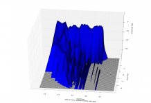
 csd,-40db,gate=5.33ms,risetime=0.02ms,nfft=1024.jpg131.9 KB · Views: 208
 -
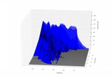
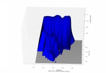
 csd,-40db,gate=5.33ms,risetime=0.15ms,nfft=1024.jpg131.3 KB · Views: 210
 -
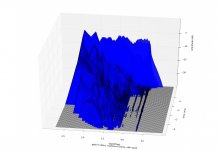
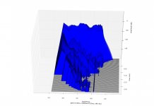
 csd,-40db,gate=5.33ms,risetime=0.5ms,nfft=1024.jpg140.4 KB · Views: 208
 -
 csd,-40db,gate=5.33ms,risetime=0.5ms,nfft=512.jpg128.4 KB · Views: 58
 -
 csd,-40db,gate=5.33ms,risetime=0.15ms,nfft=512.jpg127.4 KB · Views: 54
 -
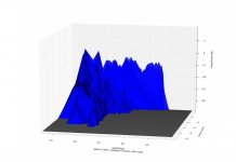
 csd,-25db,gate=5.33ms,risetime=0.02ms,nfft=512.jpg116.3 KB · Views: 49
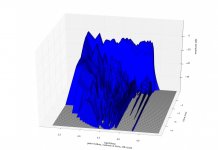
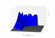
Here are some responses with a -24dB scale. They make the midrange look much more benign. Frequency response looks a little crazy here. Keep in mind the aspect ratio and that the x-axis is plotting from 100Hz to 100Khz.
Attachments
Cool...
Is that a vintage Hartke up there?
Would make a cool clock on the wall if it is no longer functional...
Later,
Wolf
Is that a vintage Hartke up there?
Would make a cool clock on the wall if it is no longer functional...
Later,
Wolf
- Status
- Not open for further replies.