The traditional grid-dip meter is an old favorite of the DIY/Ham community: initially, it was a tube-based instrument, but in the sixties it has been modernized with FETs or BJTs whilst retaining the same basic operating principles.
It is a variable-frequency oscillator using a number of pluggable coils and a variable capacitor to cover the frequency range, typically ~200kHz to 100MHz.
The coil is external and can be coupled to a tuned circuit to be tested.
The grid/gate/base of the oscillator has its bias connected to a galvanometer: the oscillation combined with the grid or base rectification generates a current dependent on the activity of the oscillator.
Typically, the bias is adjusted to be on the verge of oscillation, and the frequency is varied with the coil lightly coupled to the resonant circuit under test. When the frequency of the oscillator coincides with that of the tuned circuit, a significant amount of energy is siphoned by the external circuit, leading to a sudden dip in the amplitude of the oscillations.
This dip shows on the galvanometer, and by reading the calibrated frequency dial, it is possible to know the tuning frequency with a reasonable accuracy.
The measurement process is slow and not very deterministic, but the instrument is cheap, and can have other uses, like a frequency generator, which is why it was popular for a very long time.
The alternative I propose emulates the main function of a grid-dip (determination of the resonant frequency), but uses totally (if not opposite) principles: the circuit does not oscillate until it is presented with a tuned circuit.
The circuitry of the pseudo-grid dip is essentially aperiodic, meaning it works for all frequencies without coil change or manual tuning: as soon as a tuned circuit is presented, it oscillates at its resonant frequency.
How does it work?
The oscillator is amplifier-based, and conditional on the external tuned circuit.
"Canonical" oscillators like those used in grid-dips are based on a 3-terminal active device (tube, FET, BJT, etc.) and three reactive elements: two capacitors and one inductor results in a Colpitts configuration, and two inductors and one capacitor a Hartley.
Other types of oscillator are based on a quadripole and a frequency-selective network: a typical example is the diff-amp oscillator.
This circuit is quadripole-based, but the selective network is external and also acts as a gate: in its absence, the positive feedback is completely absent.
In addition, the external circuit is only inductively coupled, to mimic the original instrument
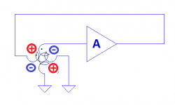
This sketch outlines the electrical configuration:
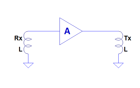
Nothing is particularly unusual: it is an amplifier looped back on itself, except the positive feedback is nonexistent, because the input and output inductors are not coupled.
Thus, such a circuit has no chance to oscillate, but then, where is the catch?
The answer is in the geometric configuration of the coils: they are magnetically orthogonal, meaning their coupling coefficient is zero.
This is a more faithful representation of the physical configuration:

It is now obvious that no coupling can exist between the Tx and Rx coils, but how can such a configuration oscillate in the end?
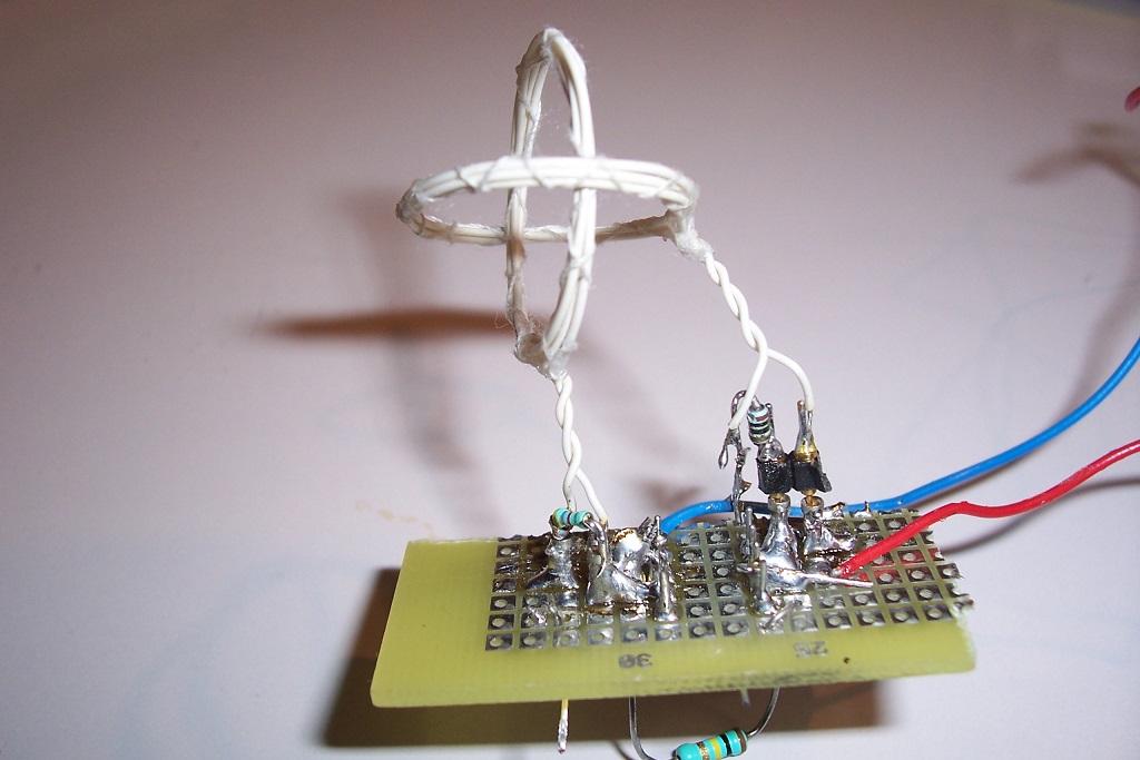
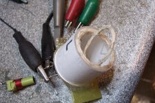
The two coils divide the space into 4 quadrants: a picture of the prototype should make things clearer:
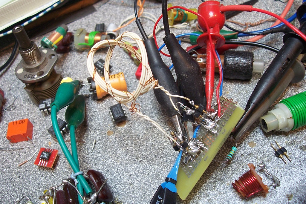
The two coils of this prototype are ring-shaped, about 27mm dia, and comprise 6 turns of wire-wrapping wire. Their inductance is a little under 2µH.
If a tuned circuit is present in any of the quadrants, it will be able to interact with both inductors, because it will not be orthogonal.
The transmission coil can induce a resonance in the tuned circuit, and in turn, the current in its inductor will couple to the reception coil.
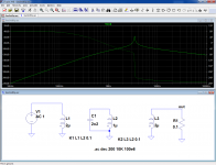
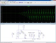
This is shown in this simulation:
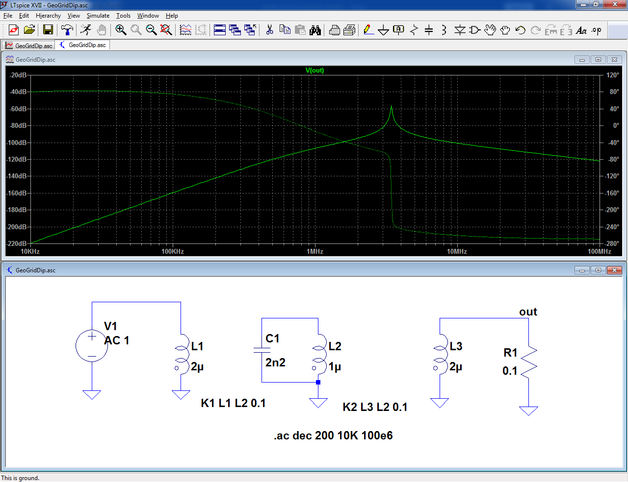
Coupling coefficients are only defined for L1/L2 and L2/L3, yet the signal from L1 manages to reach L3.
To summarize, the Tx and Rx coils do not see each other directly, but the Tx coil can “illuminate” the tuned circuit, which then becomes visible to the reception coil.
It is a variable-frequency oscillator using a number of pluggable coils and a variable capacitor to cover the frequency range, typically ~200kHz to 100MHz.
The coil is external and can be coupled to a tuned circuit to be tested.
The grid/gate/base of the oscillator has its bias connected to a galvanometer: the oscillation combined with the grid or base rectification generates a current dependent on the activity of the oscillator.
Typically, the bias is adjusted to be on the verge of oscillation, and the frequency is varied with the coil lightly coupled to the resonant circuit under test. When the frequency of the oscillator coincides with that of the tuned circuit, a significant amount of energy is siphoned by the external circuit, leading to a sudden dip in the amplitude of the oscillations.
This dip shows on the galvanometer, and by reading the calibrated frequency dial, it is possible to know the tuning frequency with a reasonable accuracy.
The measurement process is slow and not very deterministic, but the instrument is cheap, and can have other uses, like a frequency generator, which is why it was popular for a very long time.
The alternative I propose emulates the main function of a grid-dip (determination of the resonant frequency), but uses totally (if not opposite) principles: the circuit does not oscillate until it is presented with a tuned circuit.
The circuitry of the pseudo-grid dip is essentially aperiodic, meaning it works for all frequencies without coil change or manual tuning: as soon as a tuned circuit is presented, it oscillates at its resonant frequency.
How does it work?
The oscillator is amplifier-based, and conditional on the external tuned circuit.
"Canonical" oscillators like those used in grid-dips are based on a 3-terminal active device (tube, FET, BJT, etc.) and three reactive elements: two capacitors and one inductor results in a Colpitts configuration, and two inductors and one capacitor a Hartley.
Other types of oscillator are based on a quadripole and a frequency-selective network: a typical example is the diff-amp oscillator.
This circuit is quadripole-based, but the selective network is external and also acts as a gate: in its absence, the positive feedback is completely absent.
In addition, the external circuit is only inductively coupled, to mimic the original instrument
This sketch outlines the electrical configuration:
Nothing is particularly unusual: it is an amplifier looped back on itself, except the positive feedback is nonexistent, because the input and output inductors are not coupled.
Thus, such a circuit has no chance to oscillate, but then, where is the catch?
The answer is in the geometric configuration of the coils: they are magnetically orthogonal, meaning their coupling coefficient is zero.
This is a more faithful representation of the physical configuration:
It is now obvious that no coupling can exist between the Tx and Rx coils, but how can such a configuration oscillate in the end?
The two coils divide the space into 4 quadrants: a picture of the prototype should make things clearer:
The two coils of this prototype are ring-shaped, about 27mm dia, and comprise 6 turns of wire-wrapping wire. Their inductance is a little under 2µH.
If a tuned circuit is present in any of the quadrants, it will be able to interact with both inductors, because it will not be orthogonal.
The transmission coil can induce a resonance in the tuned circuit, and in turn, the current in its inductor will couple to the reception coil.
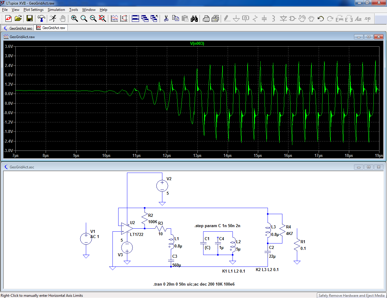
This is shown in this simulation:
Coupling coefficients are only defined for L1/L2 and L2/L3, yet the signal from L1 manages to reach L3.
To summarize, the Tx and Rx coils do not see each other directly, but the Tx coil can “illuminate” the tuned circuit, which then becomes visible to the reception coil.
Attachments

The principle of the pseudo-grid-dip look simple enough, but as always, the devil is in the details.
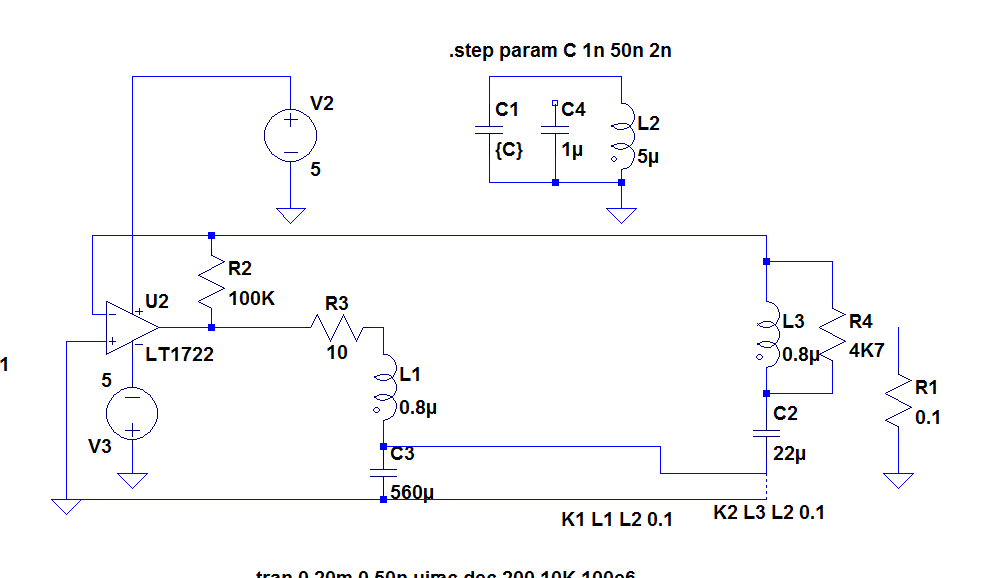
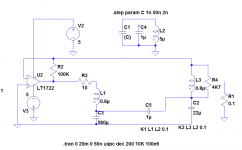
In this sim, you may notice some peculiar details:

L1 is driven by a voltage source, nothing particularly unexpected there, but the Rx coil L3 is ~shorted, and operates in current mode. This is no coincidence: to oscillate, the circuit needs to satisfy the obvious gain condition, G>1, but the phase condition is equally important: there has to be a frequency where G is >1, and φ=0 simultaneously, and preferably at the resonant frequency, otherwise it defeats the whole point of the project.
The reason for those driving conditions is that at the resonance, the tuned circuit introduces a 90° phaseshift.
It is thus necessary to adopt a hybrid Rx-Tx scheme: one of the ports has to be current controlled, and the other voltage controlled.
Here, the input (Tx) is voltage-driven, meaning the current (and mag flux) is in quadrature (delayed).
At the resonance, the tuned circuit creates an additional 90° phaseshift, because the resonance voltage overwhelms the initial induced voltage (assuming a sufficient Q factor and loosely coupled circuits).
And finally, the current induced in L3 is in phase with L2, meaning the two previous phaseshifts cancel one another.
The other option, current drive + voltage sensing is also theoretically possible, but is problematic from a practical point of view: when the frequency is lowered, the current drive remains identical, but the dΘ/dt in the tested coil is proportionately lower, as is the induced emf at the output. This results in a loss of gain.
With a voltage drive, the current is inversely proportional to the frequency, and this automatically compensates for the loss of gain.
The voltage drive/current sense has another advantage: both coils operate in low-impedance, quasi-shorted conditions, meaning their parasitic parameters like parallel capacitance become almost irrelevant: with the 2µH coils of the prototype, normal operation remains possible at more than 40MHz, which wouldn't be possible otherwise.
In reality, things are somewhat more complicated, because components are imperfect, especially coils, but one thing at a time....
To be continued...
In this sim, you may notice some peculiar details:
L1 is driven by a voltage source, nothing particularly unexpected there, but the Rx coil L3 is ~shorted, and operates in current mode. This is no coincidence: to oscillate, the circuit needs to satisfy the obvious gain condition, G>1, but the phase condition is equally important: there has to be a frequency where G is >1, and φ=0 simultaneously, and preferably at the resonant frequency, otherwise it defeats the whole point of the project.
The reason for those driving conditions is that at the resonance, the tuned circuit introduces a 90° phaseshift.
It is thus necessary to adopt a hybrid Rx-Tx scheme: one of the ports has to be current controlled, and the other voltage controlled.
Here, the input (Tx) is voltage-driven, meaning the current (and mag flux) is in quadrature (delayed).
At the resonance, the tuned circuit creates an additional 90° phaseshift, because the resonance voltage overwhelms the initial induced voltage (assuming a sufficient Q factor and loosely coupled circuits).
And finally, the current induced in L3 is in phase with L2, meaning the two previous phaseshifts cancel one another.
The other option, current drive + voltage sensing is also theoretically possible, but is problematic from a practical point of view: when the frequency is lowered, the current drive remains identical, but the dΘ/dt in the tested coil is proportionately lower, as is the induced emf at the output. This results in a loss of gain.
With a voltage drive, the current is inversely proportional to the frequency, and this automatically compensates for the loss of gain.
The voltage drive/current sense has another advantage: both coils operate in low-impedance, quasi-shorted conditions, meaning their parasitic parameters like parallel capacitance become almost irrelevant: with the 2µH coils of the prototype, normal operation remains possible at more than 40MHz, which wouldn't be possible otherwise.
In reality, things are somewhat more complicated, because components are imperfect, especially coils, but one thing at a time....
To be continued...
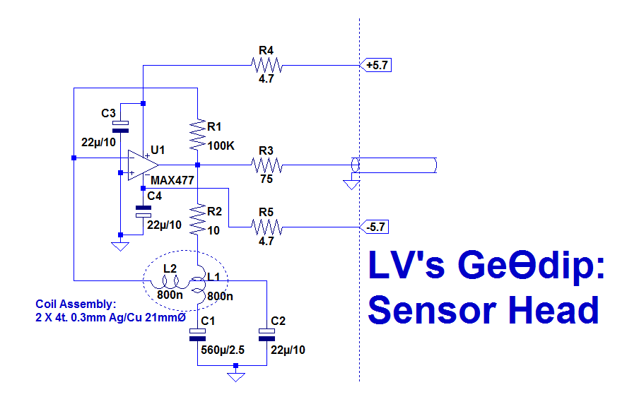
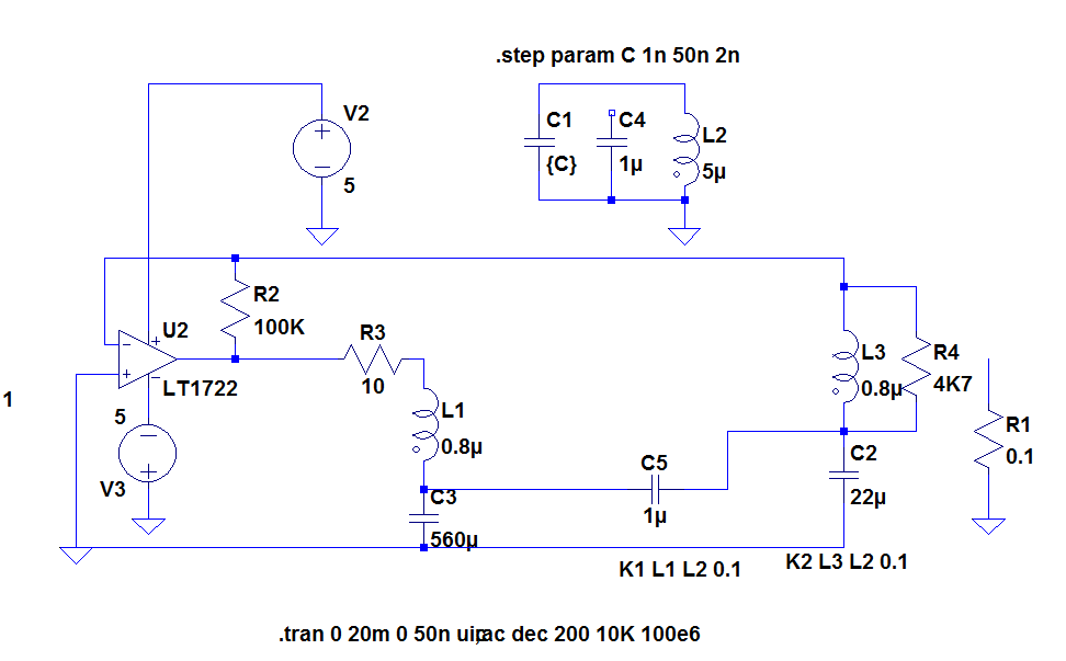
Here is the implementation I opted for:
It uses a fast opamp as a gain block, which is an easy/lazy solution: in fact, there is no need for the amplifier to be operational, as the circuit does not require closed-loop stability or DC accuracy, but it is convenient and nowadays, it becomes difficult to find general-purpose, non-operational amplifiers.
A non-op amplifier has no restrictions on its high-frequency gain or other characteristics, and can be simpler for the same level of performance, but they are a rarity, whilst HF opamps are ubiquitous.
I chose a LT1722 in the sim, but in practice I tested many other types: OPA620, AD849, CLC420 and MAX477 in VFA.
The circuit can also work with CFA types, and I tested a number of them: AD811, EL2020, EL2120 and EL2160. I expected them to work better than VFA's in this role, but I was disappointed: they required a modification of the coupling caps configuration to ensure their LF stability, and their gain was inferior, making the circuit less sensitive.
The highest performer was the AD849, but it had annoying quirks, in particular a DC shift in the presence of a HF signal which made its stabilization a nightmare.
I tried my my best to tame it, but in the end I gave up and opted for the MAX477, which has inferior performances but is much more docile.
The practical circuit needs some arrangements with the theory: the main one is the series resistor, R3.
It is required, because at low frequencies the reactance of the 0.8µH coil is tiny and acts as a short at the output of the opamp.
This is not healthy for the opamp itself, and even if it tolerates it, the signal recovered becomes too small to be reliably detected or measured.
The presence of the resistor changes the phase characteristic below a certain frequency, and this modifies the condition of oscillation: below 1.5~2MHz, the phase becomes reversed, meaning the tuned circuit has to be presented to another quadrant of the coil assembly.
There is no gap however: between 1.5 and 2MHz, the circuit oscillates indifferently in both quadrants.
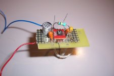
This is the circuit updated with the smaller, 0.8µH coils (4 turns, 21.5mm dia.):

I have retained the "armillary sphere" coil configuration: it is the simplest and most obvious (many others also result in a zero coupling), but it looks well suited for the intended purpose.
Here it is, enclosed in its protective plastic shell:

It uses a fast opamp as a gain block, which is an easy/lazy solution: in fact, there is no need for the amplifier to be operational, as the circuit does not require closed-loop stability or DC accuracy, but it is convenient and nowadays, it becomes difficult to find general-purpose, non-operational amplifiers.
A non-op amplifier has no restrictions on its high-frequency gain or other characteristics, and can be simpler for the same level of performance, but they are a rarity, whilst HF opamps are ubiquitous.
I chose a LT1722 in the sim, but in practice I tested many other types: OPA620, AD849, CLC420 and MAX477 in VFA.
The circuit can also work with CFA types, and I tested a number of them: AD811, EL2020, EL2120 and EL2160. I expected them to work better than VFA's in this role, but I was disappointed: they required a modification of the coupling caps configuration to ensure their LF stability, and their gain was inferior, making the circuit less sensitive.
The highest performer was the AD849, but it had annoying quirks, in particular a DC shift in the presence of a HF signal which made its stabilization a nightmare.
I tried my my best to tame it, but in the end I gave up and opted for the MAX477, which has inferior performances but is much more docile.
The practical circuit needs some arrangements with the theory: the main one is the series resistor, R3.
It is required, because at low frequencies the reactance of the 0.8µH coil is tiny and acts as a short at the output of the opamp.
This is not healthy for the opamp itself, and even if it tolerates it, the signal recovered becomes too small to be reliably detected or measured.
The presence of the resistor changes the phase characteristic below a certain frequency, and this modifies the condition of oscillation: below 1.5~2MHz, the phase becomes reversed, meaning the tuned circuit has to be presented to another quadrant of the coil assembly.
There is no gap however: between 1.5 and 2MHz, the circuit oscillates indifferently in both quadrants.
This is the circuit updated with the smaller, 0.8µH coils (4 turns, 21.5mm dia.):
I have retained the "armillary sphere" coil configuration: it is the simplest and most obvious (many others also result in a zero coupling), but it looks well suited for the intended purpose.
Here it is, enclosed in its protective plastic shell:
Attachments

Too complex IMHO. A simple triode (or a JFET) plus some resistors, inductors and capacitors do the job.
Complexity is relative: maybe it looks more complex if you put the two raw BOM's side by side (and that's not even certain, because the GeoDip is really quite simple in fact, and it does not need multiple coils and their sockets, the galvanometer, VC and other paraphernalia), but apart from the two-coil assembly, the components are mere commodities.
Fast opamps were deemed high-tech 20 years ago, but now they are common-place, and I successfully tested a number of them.
You also have to consider what you get for the complexity, real or perceived.
Regarding the convenience/ease of use, there is no competition possible compared to a traditional dip-meter.
With the traditional instrument, you first need to select one of the coils, then explore slowly the frequency range. When you have found a dip, you then read the frequency on the scale corresponding to the coil.
If you took the wrong coil, you have to take another round.
With the GeoDip, the operation is static and the result is immediate: bring the tuned circuit close to the coil head, and read the result on a frequency meter.
Nothing to scan/explore, no coil to change.
Of course, it is not a standalone instrument: you need to connect a frequency-meter to its output, but that's an instrument many hams and DIYers already have, and it would be possible to include a frequency-meter: that's what I am going to do.
Another aspect to consider is the performance.
A typical classical dip-meter has a range of ~1000:1 it could be 100kHz to 100MHz, or 150kHz to 150MHz, or even 100kHz to 150MHz, but not much more.
My GeoDip prototype has oscillated from 1.35kHz to 136MHz: a range of 100,000:1 or 100 times better.
With the MAX477, 136MHz is probably very close to the absolute limit: at 140MHz, it hits an insurmountable wall.
The lower frequency limit could certainly be extended: I just tested down to 1.35kHz, because the coil and cap combination tested happen to be there, but frequencies lower than 1kHz are probably reachable.
The AD849 was able to reach much higher frequencies and still worked at 1.35kHz, but it was a stinker.
It is a relatively old circuit though, and I expect more modern chips to be HF capable and well-behaved.
A traditional dip-meter is low-frequency limited: variable capacitors have 300 ~ 500pF, and to reach frequencies much lower than 100kHz, the coil needs to be large, but this means a large self-capacitance which limits the ratio attainable.
The GeoDip circuitry is practically aperiodic, and reaches frequencies in the kHz range easily.
The coil assembly looks complicated, but it isn't really, and it is fixed: you only need one for all the frequencies.
Two times 4 turns glued in an orthogonal position is not really difficult, and the exact size or number of turns is not critical.
The only critical aspect is the orthogonality, but it is easy to test and to glue in place.
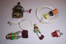
Here is a random selection of some of the tuned circuits I (successfully) used for the tests:

Fast opamps were deemed high-tech 20 years ago, but now they are common-place, and I successfully tested a number of them.
You also have to consider what you get for the complexity, real or perceived.
Regarding the convenience/ease of use, there is no competition possible compared to a traditional dip-meter.
With the traditional instrument, you first need to select one of the coils, then explore slowly the frequency range. When you have found a dip, you then read the frequency on the scale corresponding to the coil.
If you took the wrong coil, you have to take another round.
With the GeoDip, the operation is static and the result is immediate: bring the tuned circuit close to the coil head, and read the result on a frequency meter.
Nothing to scan/explore, no coil to change.
Of course, it is not a standalone instrument: you need to connect a frequency-meter to its output, but that's an instrument many hams and DIYers already have, and it would be possible to include a frequency-meter: that's what I am going to do.
Another aspect to consider is the performance.
A typical classical dip-meter has a range of ~1000:1 it could be 100kHz to 100MHz, or 150kHz to 150MHz, or even 100kHz to 150MHz, but not much more.
My GeoDip prototype has oscillated from 1.35kHz to 136MHz: a range of 100,000:1 or 100 times better.
With the MAX477, 136MHz is probably very close to the absolute limit: at 140MHz, it hits an insurmountable wall.
The lower frequency limit could certainly be extended: I just tested down to 1.35kHz, because the coil and cap combination tested happen to be there, but frequencies lower than 1kHz are probably reachable.
The AD849 was able to reach much higher frequencies and still worked at 1.35kHz, but it was a stinker.
It is a relatively old circuit though, and I expect more modern chips to be HF capable and well-behaved.
A traditional dip-meter is low-frequency limited: variable capacitors have 300 ~ 500pF, and to reach frequencies much lower than 100kHz, the coil needs to be large, but this means a large self-capacitance which limits the ratio attainable.
The GeoDip circuitry is practically aperiodic, and reaches frequencies in the kHz range easily.
The coil assembly looks complicated, but it isn't really, and it is fixed: you only need one for all the frequencies.
Two times 4 turns glued in an orthogonal position is not really difficult, and the exact size or number of turns is not critical.
The only critical aspect is the orthogonality, but it is easy to test and to glue in place.
Here is a random selection of some of the tuned circuits I (successfully) used for the tests:
Attachments
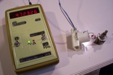
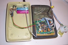
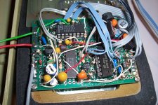
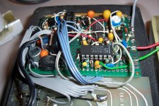
I have built the prototype into a real, usable test instrument:
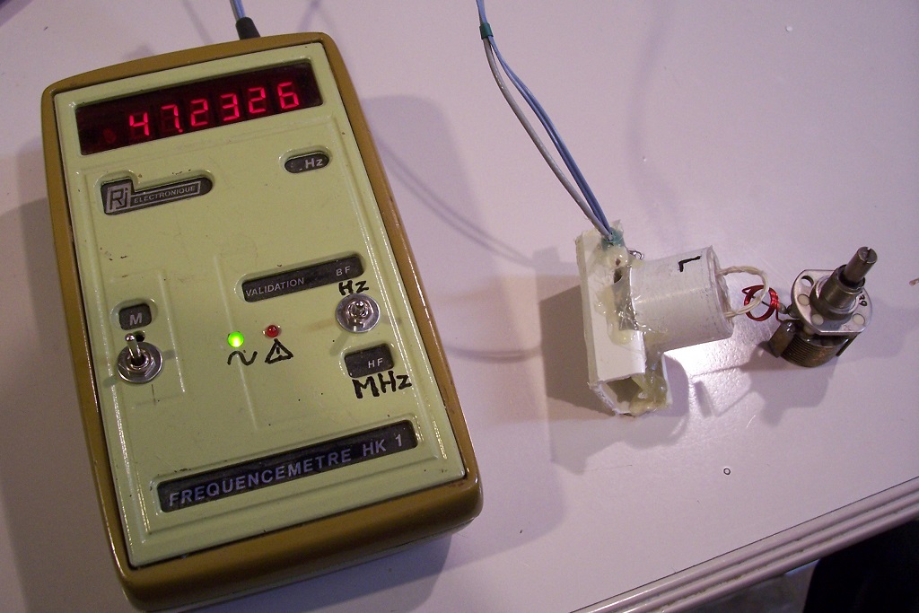
It is grafted inside an old, worthless frequency-meter for convenience and includes all the necessary bells and whistles to make it comfortable to use and reliable.
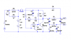
Here is the schematic of the most important part, the sensor head:
The rest will follow soon
It is grafted inside an old, worthless frequency-meter for convenience and includes all the necessary bells and whistles to make it comfortable to use and reliable.
Here is the schematic of the most important part, the sensor head:
The rest will follow soon
Attachments

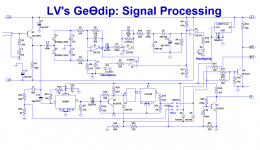
Some explanations about the signal detection: it looks overly complicated, but for good reasons.
LC oscillators can be affected by squegging, and this one is no exception.
Squegging is a form of semi-chaotic relaxation LF suboscillation that modulates the base frequency.
It is generally caused by an excess of positive reaction: oscillations build up sufficiently to shift the DC bias point, because of grid/gate/base rectification, driving the oscillator into cutoff, but as long as there is room for increased amplitude, the buildup continues until saturation occurs. At that point, the bias shift continues to increase until even class C oscillations are no more sustainable.
Oscillations then cease, and the oscillator needs some time to recover and oscillate again.
The whole process then begins again and a new cycle starts.
Sometimes, this condition is induced on purpose, as for superregenerative receivers (the process is partly chaotic, and very sensitive to initial conditions), but it is generally an annoyance.
With the Geodip, the feedback conditions vary hugely, meaning squegging is a possibility.
The MAX477 is particularly well-behaved, and squeggs only occasionnaly (I'd say ~2% of the times), but it is important to detect the condition: I built the Geodip as a standalone instrument, with no monitoring output, and the frequency-meter will average the frequency, meaning it will miss a number of cycles when squegging occurs.
The squegging detection is made by detecting LF modulation over the already detected DC signal.
Here, the situation is complicated by the fact that the Geodip operates down to the kHz level, and squegging rate can be as high as a few hundred Hz.
For that reason, U1 operates as a full-wave, frequency-doubling detector to minimize the ripple. U2 amplifies any modulation which is detected by U4 and lights the warning LED.
When squegging is signalled, one just has to move the tuned circuit back slightly, to reduce the coupling and the positive reaction.
Normally, the red LED flashes briefly at the transitions, when the oscillations start or end (unless you have Parkinson's disease, of course)
The frequency range selection is a mess, because I wanted to use a simple, center-off switch and at the same time keep a logical progression, with the 10MHz in the middle.
That's anecdotal, because the frequency measuring section is purely illustrative, and based on the contents of my junk-box: the ICs are hopelessly obsolete.
I used a 300MHz prescaler because I intend to upgrade the sensor with a better opamp than the relatively old MAX477: I hope I'll be able to reach somewhere between 200 and 300MHz
This is the power supply:
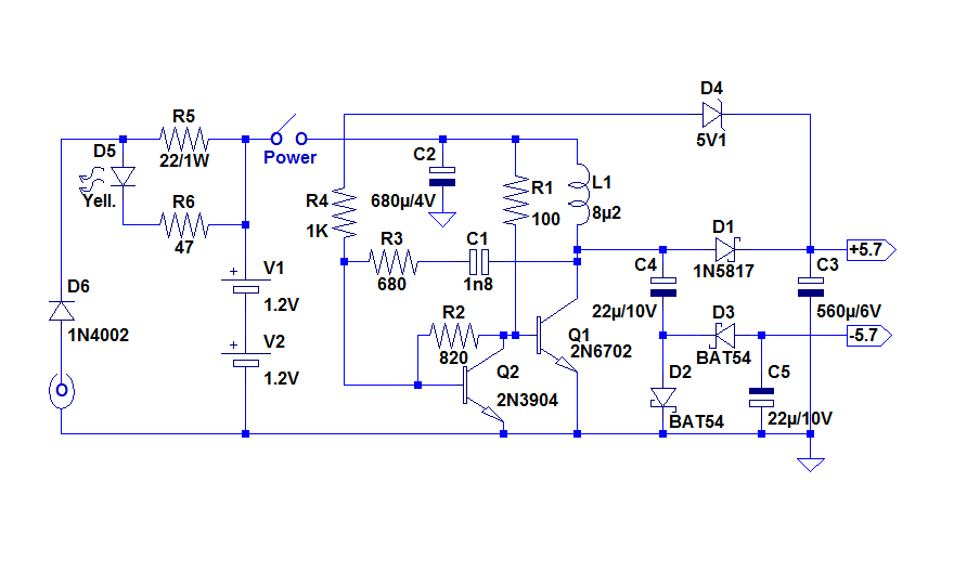
A DC-DC converter supplies everything, which looks radical but is completely logical: a converter is necessary anyway to generate the negative supply, and the difference between a low-power crude converter and a medium-power crude converter is just in the components size: slightly bigger.
So, instead of using a 200mW converter and 5 NiMh cells, I used 2 cells and a 2W converter.
The converter is a very low-tech, self-oscillating one, based on the FB topology.
The frequency of operation is comprised between 80 and 100kHz.
It is crudely regulated.
I used a 2N6702 (with the mounting tab snipped) as power element, which should be completely unsuitable based on the datasheet, but the ones in my stock shine, and work remarkably well for a largish, HV type (other sources would probably behave dismally).
A more sensible choice would be a ZTX---, but I had no suitable type in my drawers.
The average output power is ~2W (the vintage display, prescalers and analogue circuits are power-hungry), resulting in a 1A consumption on the 2.4V input side.
When the oscillator runs at its 145MHz maximum, it rises to almost 1.5A, but this is relatively unimportant: with ~3Ah elements, the autonomy is still 2~3h, which is ample considering the type of use of such an instrument.
Initially, I had used a standard drum-core choke for the 8.2µH storage coil, but the open magnetic circuit leaked too much in the environment.
I first changed the other 8.2µH RF choke for a custom-wound one on a closed magnetic core (a ferrite bead), but the sensor head was also affected, and I had to wind the power choke on a miniature, completely closed potcore.
This solved the issues.
Attachments
Here is a small video showing the Geodip tested with a number of tuned circuits, from 1300Hz to >100MHz.
YouTube
It can of course test and ping any resonant circuit-based device, including RFID tags, NFC interfaces, wireless power systems, transponders, anti-theft devices, E-tickets, etc.
The "normal" operating mode, as described in the first post, starts at ~1.5MHz, but it doesn't extend to the maximum frequency: above ~65MHz, there is another phase inversion, probably caused by the phaseshift in the opamp and the parasitics of the sensor coils.
The maximum frequency is 145MHz, but the tuned circuit needs to pushed inside the "armillary sphere".
For the low-frequencies too, at 1.3kHz, the tuned circuit has to be inside the sphere because of the very low Q.
The display only has 6 digits, meaning that for frequencies >100MHz, the overrange LED acts as a "1". I didn't want to add a range just for that
Some additional information:
Ideally, the size of the sensor coils should broadly match that of the tested device.
That is valid for any magnetically-coupled device: it maximizes the common field and thus the coupling.
If the main interest is E-tags, E-tickets, wireless or NFC interfaces for example, a diameter of several cm would be ideal.
For general VHF/ham applications, 1cm would be more appropriate.
The 21mm I opted for is an excellent general-purpose choice: as you can see in the video, it easily adapts to large and small coils, from a few mm to more than 10cm.
As I mentioned earlier, other configurations are possible: an off-centered armillary sphere for example, to make more room for the DUT or overlapping loops in the same plane, as in metal detectors.
In fact, all the configurations used in IB metal detectors would be usable (but not necessarily practical in a grid-dip meter).
The number of turns should suit the frequency range: here again, 4 turns is OK for a general purpose instrument, but for VHF/UHF application, 2 or even 1 turns would be preferable.
For lower frequencies, a larger number is of course preferable.
One could also make pluggable sensor assemblies, but this would defeat the main purpose of the project: one-size-fits-all for a > 1 : 105 frequency range.
This grid-dip substitute performs the main function of such an instrument, and does it more simply and effectively, but conventional grid-dips have a number of other uses: they can act as a crude, uncalibrated signal generator for example.
This emulation can only generate a signal when coupled to a resonating circuit, and in some instances, it might be possible: as an exciter in the low power stages of a transmitter for example.
Otherwise, one would need to couple an additional tank to make a generator, but this would be cumbersome and unpractical.
A grid-dip on the verge of oscillation can make a sensitive, tuned field-strength meter. This substitute is an extremely sensitive magnetic sniffer (= field-strength meter), and it does not need to be tuned: it displays the detected frequency directly.
If "difficult" amplifiers like CFA's are used, VLF instabilities can occur.
To stabilize the circuit, it is necessary to use a different coupling caps configuration.
This is the most radical (and effective), but it will limit the LF performance:
A less violent (and less effective) approach will leave the LF performance mostly intact, but it has to be adapted to the opamp used:
Attachments
The Geodip concept has interesting "philosophical" implications: it can detect a tuned network in its frequency and space range, but it does so without emitting or receiving any apparent signal.
Conventional devices like card readers or grid-dip meters need to send a stimulus, a signal of some kind.
By contrast, when the Geodip is idle, it is as inert and passive as a lump of wood or a concrete block: it emits absolutely no detectable signal.
The target too is completely passive and inert, yet when they are within range, the Geodip wakes up and emits a signal at the correct frequency.
Imagine a similar situation in the optical domain: someone sits inside a completely dark room: not a single visible photon is present.
A color sample is then unveiled; it is just a pigment and emits no light of its own, yet in the complete darkness the person can tell exactly what color is the sample.
Intriguing, isn't it?
Of course, there is no magic: it is just a peculiar type of oscillator having its elements physically separated, but it is nevertheless amazing.
The concept could be used to make "stealth" reader: a regular card reader or anti-theft system betrays itself by permanently emitting an exploratory field.
With the Geodip, the oscillation only appears when the two elements are close enough.
Your analysis is ignoring thermal noise and amplifier noise. You optical analogy isn't realistic as optical light is not thermally activated in normal situtations. Substitute far infra-red (which is thermally active at normal temps) and you'll realize there is no "completely dark room", all objects are glowing with their
own colour spectrum and lots of photons are always present!
The amplifier is broadcasting its noise to the output coil, the tuned circuit is emiting and receiving em radiation constantly with its environment, ie has a colour (unless its completely reactive, unlikely). The correlation the amp sees
between the input coil signal and the noise it sends to the output coil is going to lead to build up an oscillation favoured by the tuned circuit.
Yes, I agree completely, and I mentioned it myself:
The starting mechanism is the same as for any other oscillator, but having the elements physically separated gives an impression of weird, spooky effects (perfectly explainable in a hard, rational way though)
Of course, there is no magic: it is just a peculiar type of oscillator having its elements physically separated, but it is nevertheless amazing
The starting mechanism is the same as for any other oscillator, but having the elements physically separated gives an impression of weird, spooky effects (perfectly explainable in a hard, rational way though)
- Home
- Design & Build
- Equipment & Tools
- A geometry-based grid-dip meter emulation