In the last few days off, I have been somewhat confused and have tried to collect enough reasonable data for a possible replacement circuit using the usual home remedies. I don't know whether I succeeded or whether I was able to develop a common thread; the more diagrams one plot, the more confused the scenario becomes. I deliberately left out the interesting mechanical side, because how can one approach it reasonably well with home remedies? Of course one can think about the elastic side between the cantilever and tip and the plastic disk, but on average we always come to a conclusion, reso fo is always less than 35kHz and the cutoff fc moves from 61kHz to 32kHz ... outside to inside.
Perhaps we can develop a test procedure, a common thread, together at this point.
Perhaps we can develop a test procedure, a common thread, together at this point.
Attachments

One of the driving forces for me is the question of whether the model is really independent of the load, the later operating case.
That's why I approached it with different measuring currents by recording a series for R1=Rload -> 547Ohm, 4k7, 22k, 47k, 220k. The values of the model simply cannot be completely independent of the a) method and the b) measurement current or voltage.
Wouldn't it be better to work with a constant current flow? Which absolute value is the correct or best for the present mm-pickup, the DUT?
With a measuring bridge (is it a bridge method???) I get fantastic results for five frequencies, but how does the coil behave electrically above the resonance maximum? Does a parallel resonance exist in reality? In my first measurements, it shifted to the right with decreasing load (i.e. R1 becomes larger).
_____________________
If anyone would like to have the (erroneous) raw data, i.e. the voltage measurements, I will be happy to send them to you by PM.
One can follow or trace my loose thoughts and steps in the PDF above.
Attachments
Last edited:

This may mean, however, that the derived model can only be tolerant of load changes to a certain degree.
In other words, it is often referred to as a scope of validity. In this case, the question is abbreviated to: dV valid, df & fmax valid and dRload, dCpload. This applies to the model in question.
In a nutshell: Is my (or another) model sufficiently accurate to correctly model different load cases as a resulting transfer function?
Sorry, but I'm thinking about measuring the coil data until I get a converging result.
If one keep the voltage at R1 constant by adjusting the source voltage to the test frequency (point), a constant current flows through the pickup. But what is the optimum value? A value that cooperates well with the later application (i.e. Rload)? Is it 50µApp with 20kOhm or better only 25µApp at 40kOhm ..!?
To be honest, the topic is not as trivial as one (or I) thought if one want to cover a frequency range of up to 1 MHz.
HBt.
Attachments
Why all the magic?
Because the known (electrical) models (the components and their arrangement) cannot possibly represent the range between 100kHz and 1MHz correctly.
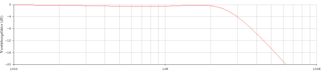
Apparently this leads to the result that we don't simulate the typical (slight) bathtub in the upper midrange (or lower treble) - the lumped model can't do that. At least that seems to be the case.
But until I have an absolutely trustworthy electrical model for the coil that reproduces this enormous band over five decades, I cannot draw any reliable conclusions about an electrical replacement model of the cantilever (via the subtractive route).
In practice, however, this is not important because of the mechanical interaction with the plastic disk and the contact force and contact surface. Two really incisive limits, referred to as fo_mech (parallel resonance) and the wandering fc_mech (series resonance), limit our sensible range of application. The frequency range, the band - classically, this cut-off frequency is set at least one octave lower 30kHz/2 would now be 15kHz. Our resulting play with Rload and Cload leads to a combination (i.e. a higher order of some kind), i.e. an optimum cut-off frequency in between.
It is a game with the moving masses, but above all with the resulting contact surface (the diamond with its cut and dimensions) and the contact force. We can push this to the right as long as the scanning capability remains safe. The responsible cutter will electrically limit the highest signal frequency to less than 20 kHz anyway.
HBt.
Because the known (electrical) models (the components and their arrangement) cannot possibly represent the range between 100kHz and 1MHz correctly.
Apparently this leads to the result that we don't simulate the typical (slight) bathtub in the upper midrange (or lower treble) - the lumped model can't do that. At least that seems to be the case.
But until I have an absolutely trustworthy electrical model for the coil that reproduces this enormous band over five decades, I cannot draw any reliable conclusions about an electrical replacement model of the cantilever (via the subtractive route).
In practice, however, this is not important because of the mechanical interaction with the plastic disk and the contact force and contact surface. Two really incisive limits, referred to as fo_mech (parallel resonance) and the wandering fc_mech (series resonance), limit our sensible range of application. The frequency range, the band - classically, this cut-off frequency is set at least one octave lower 30kHz/2 would now be 15kHz. Our resulting play with Rload and Cload leads to a combination (i.e. a higher order of some kind), i.e. an optimum cut-off frequency in between.
It is a game with the moving masses, but above all with the resulting contact surface (the diamond with its cut and dimensions) and the contact force. We can push this to the right as long as the scanning capability remains safe. The responsible cutter will electrically limit the highest signal frequency to less than 20 kHz anyway.
HBt.
The crux of the matter is the following:
R||L||C assumes that all losses can be expressed by R, i.e. sublimated. However, the C is only formed by the resulting electric field and is absolutely not an ideal component. This C in our lumped model must also be lossy (on its own and not in combination, the combination effect only occurs later in the course of the overall model formation), just like the coil that is actually present, with its N windings around the soft magnetic core. Losses now occur here in the permanent alternation of the magnetic field, including the notorious eddy current losses. The R in the simple RLC model is divided between these two physical phenomena or energy stores, while the coil winding can still be partially divided further, leaving a C with its own R in series.
Once this hurdle has been overcome, the mutual matching of the partially divided L (coil) takes place with at least Rp||Lp + Rs&Ls. Where Rs almost always represents Rdc, the pure wire resistance of the winding.
After, or better yet, during, the modeling (the fit), the best approximation of the phase and amplitude frequency response must be continuously sought. This requires data from the future four-pole system, the transfer function without Cload, in advance.
We disregard all this if the coil (here the pickup) is characterized (using a network analyzer or bridge ... alone) but has not been examined in its later practical load case. If there were a test record that could cover all the absolutely necessary decades linearly, then we could simply put it on and let the generator (the pickup) itself tell us what it really looks like analytically (but only mechanically-electrically, in an electrical equivalent). This path is not available to us, as we all know.
However, our goal is an image with a wide range of validity in the natural habitat and working range of the transducer. What's still missing from the dream is a piezo accelerator that could set our lever arm in motion correctly (i.e., according to the record groove) (but) up to 1 MHz. A model up to 20 kHz is very easy to create; it was already possible in 1970. Unfortunately, every body vibrates, because mass has elasticity, thus acting as a damper.
Measurement setups in mechanics, including force measurement technology, are absolutely not trivial, especially not from a dynamic perspective.
So if you look at a model that has a global R and a global C parallel to the coil simulation, the fit can indeed form a two-pole in terms of magnitude, which later in the four-pole, i.e. with Rload and Cload, is reasonably correct up to just over 20kHz, but nothing more. You can never infer the mechanics with this. Theoretically, the known (new) subtraction method works. But two things are essential for this: a) the electrical generator model must really fit (up to 1MHz) and b) the test record and the sampling capability of the object under investigation must have a cutoff frequency very far to the right (e.g. 10*20kHz). Unfortunately, the latter points are all mutually exclusive.
HBt.
The extent to which the coil needs to be divided into partially valid parts can be seen from the curve of the apparent resistance, the impedance. If necessary, a polynomial and the familiar curve analysis from our school days are needed. Hence, differential equations. Derivatives. But one can plot the |Z| (and |Phi| between to timecourses) and also gain valuable clues using graphical methods.
In this spirit, I hope for a lively exchange.
Perhaps another user can contribute measurements and data to make the steps of a possible modeling transparent to other people.
In this spirit, I hope for a lively exchange.
Perhaps another user can contribute measurements and data to make the steps of a possible modeling transparent to other people.
Your electrical model and its values in post #1 look likely, although for best results you should divide modelled impedance by measured impedance and plot that as a percentage. Had I measured your cartridge, I would expect spot deviations of <10% over the five decades between model and measurement. And yes, when loaded by the wrong R and C, the electrical model does show the traditional upper mid-range dip.
The deviations are even significantly lower, provided I load (it) with 47kOhm.I would expect spot deviations of <10% over the five decades between model and measurement.
At 220kOhm, the argument and the angle no longer fit so well. And that is one of the driving reasons for the question of the general range of validity of our models.
Exactly, but lumped models that represent the parasitic capacitance as an ideal capacitor parallel to the rest often do not show it.And yes, when loaded by the wrong R and C, the electrical model does show the traditional upper mid-range dip.
It's crazy ...
Deviations in impedance, not what that impedance does to level when loaded by 47k.
And that's credit to the cartridge manufacturers for being able to manipulate their generator to be able to fit an awkward standard.
No craziness, it's measurable and predictable. Given that the six-component model fits to 200kHz, I think it's a pretty good model. More to the point, it fits much better than the old LR model.
My suggestion modifies the structure so that the last decade (0.1MHz till 1MHz) can also be mapped correctly and the later bathtub only enables the dip.

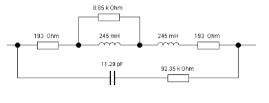
The usual structure is almost identical to the known R || L' || C form. While the L' may of course represent a coil divided into arbitrary segments, this unfortunately does not change the basic shape or curve of the resulting impedance.
But the key is the red-marked components in series connection, not as usual (alone as themseves) in parallel with the coil replacement.
This configuration naturally results in different values for the components (to simulate the impedance) than your model with only C and R in parallel to the coil inductance approximation.
Try it out with the well-known Shure V15-III model values and calculate the alternative.

Finally, the transfer function H(jOmega) must be compared, because we are interested in what comes out on the far right, i.e. at the back. The exciting question is not only which structure is better at mapping the |Z|(f), but also which one does it more correctly overall and what is necessary for this. For my suggestion we need raw data above 100k or 200k Hertz.
The usual structure is almost identical to the known R || L' || C form. While the L' may of course represent a coil divided into arbitrary segments, this unfortunately does not change the basic shape or curve of the resulting impedance.
But the key is the red-marked components in series connection, not as usual (alone as themseves) in parallel with the coil replacement.
This configuration naturally results in different values for the components (to simulate the impedance) than your model with only C and R in parallel to the coil inductance approximation.
Try it out with the well-known Shure V15-III model values and calculate the alternative.
Finally, the transfer function H(jOmega) must be compared, because we are interested in what comes out on the far right, i.e. at the back. The exciting question is not only which structure is better at mapping the |Z|(f), but also which one does it more correctly overall and what is necessary for this. For my suggestion we need raw data above 100k or 200k Hertz.
As it happens, an 8MHz impedance analyser should be arriving soon, but 200kHz ought to be adequate to determine audio parameters.
What physical justification are you offering for putting the resistor and capacitor in series? A model has to be physically justifiable.
I would point out that sample variation at spot frequencies between channels and between supposedly identical cartridges is greater than the fitting error I see between my six-component model and measurement. To my mind, that says the model is as good as it needs to be.
To identify the usual three passive components R, L & C, (up to) 100kHz is also sufficient. Of course, only if we are not interested in their behavior outside the audible range.As it happens, an 8MHz impedance analyser should be arriving soon, but 200kHz ought to be adequate to determine audio parameters.
In short:
I am looking forward to your measurements with the new (automatic) analyzer.
You are absolutely right that this is a very weighty objection - it must be taken into account. The question of the credible operational capability of both model structures has not yet been conclusively and convincingly answered. We know that the electric field and all interactions that occur must represent our component with the letter C. This C as a representative cannot be an ideal and constant component - for this reason alone we should already think about an ohmic series resistor, consider it. A physical traceability /return can take place later if the model has proven to be electrically conclusive and sound.What physical justification are you offering for putting the resistor and capacitor in series? A model has to be physically justifiable.
Are you using the use /load case as a basis - H(jOmega)_model vs. H(JOmega)_reality ?I would point out that sample variation at spot frequencies between channels and between supposedly identical cartridges is greater than the fitting error I see between my six-component model and measurement.
In practical terms, you may be absolutely right. But nothing prevents us from extending the accuracy and range of validity immeasurably in the computer, i.e. virtually.To my mind, that says the model is as good as it needs to be.
I am concerned with the safe suitability of the longitudinal structure, so that we can make credible predictions in a wide load case.
Bob C. is on the left in this spectrum and Nick S. on the right with 5k<Rload<200k. Only when we are absolutely certain and all questions have been credibly answered and physically substantiated and traced back, can the structure of the electrical model of the transducer's coil serve further purposes. For example, the possible electrical replacement modeling of the mechanical part.
HBt.
Simply put:
In the usual and already substantially extended model structures, we see a C (standing alone) parallel to the other components. This reactance will eventually short-circuit all the other components completely. This means that the impedance curve must follow the abscissa very soon, with a value of zero ohms.
And that is exactly what we see in all these cases. At the same time, we also know that this behavior can never correspond to reality. Ergo, the model is not entierely correct, of course we will never see this unless we open the window (as the frequency range) wide and look beyond the horizon.
Sometimes a partially valid, sufficient model is not enough.
That may take a while. I was given a one week lead time eight days ago, but it hasn't arrived, and I'm now being given the runaround. And once it does arrive, I'll have to learn how to talk to it from computer. No way am I recording a hundred or more impedance measurements manually. Further, I had to borrow many of the cartridges I tested, and they might no longer be available. It's a funny thing, but people are reluctant to remove a working cartridge from their turntable and lend it for testing. But I can measure the Ortofon VMS20, OM, and Super OM. I seriously doubt that going to 8MHz will reveal anything significant to audio, but the ability will be there, so it will have to be exercised.I am looking forward to your measurements with the new (automatic) analyzer.
I fit a model to the measured impedance. I deem reality to be a least squares fit to measured impedance fit that produces a residual having minimal discernible structure and a standard error <5%. You might need to brush up your statistics to follow that. What is done with that impedance later is a separate issue, but the predictions from adding load capacitance and resistance and calculating amplitude against frequency response seem plausible. I am only concerned with the transducer's electrical impedance, not how it convertes mechanical modulation into an electrical signal. One step at a time...
In a spirit of enquiry, I will see what happens if I fit to a model having a resistance in series with the capacitance. This may take some time because the algebra is quite unpleasant and it's easy to make a mistake when typing it into the spreadsheet.
Summarising: The traditional LR model fits cartridges very badly. My six-component model visibly fits impedance far better, explains where the 1970s upper mid-range dip came from, and predicts the cut-off frequency of the low-pass electrical filter correctly. It allows optimum electrical loading to be determined, and those predictions are sufficiently close to manufacturers' recommendations to be plausible. But sample variation of cartridges is significant and greater than my model's fitting error, so I judge the model to be good enough.
We know that cartridges are temperature and humidity sensitive, so I suspect that a useful electrical analogue of the mechanical system will be tricky. But that needn't stop us from making sure that we treat the electrical system correctly.
I just tried your variant of the six-component model. It can be fitted up to 200kHz but produces a very slightly higher standard error (two cartridges went from 1.5% to 1.6%). Intuitively, a resistance in series with the capacitance will cause impedance at infinite frequency to fall to a constant value, which I would argue is unlikely because I cannot see a physical justification for it, and I think that's what the increased standard error is warning. However, when the 8MHz analyser arrives, it will allow a definitive answer.
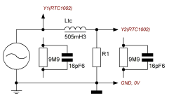
I have created another series of measurements (left coil only). With R1=20kOhm and compensated Tektronix TPP0201 probes.


Our measured value is also dependent on the operating point, which is the real, simulated load case. Here with 20kOhm and 1Vpp original source-voltage, far left! Current also as peak to peak value.


f_reso exactly 114.1kHz with 0° phaseshift.
I am very much looking forward to your new measurements, with the values of the VNA above 100kHz to n MHz. One could assume the short circuit of a prototype MM with just under 2µA(rms) as the operating point.
HBt.
Our measured value is also dependent on the operating point, which is the real, simulated load case. Here with 20kOhm and 1Vpp original source-voltage, far left! Current also as peak to peak value.
f_reso exactly 114.1kHz with 0° phaseshift.
I am very much looking forward to your new measurements, with the values of the VNA above 100kHz to n MHz. One could assume the short circuit of a prototype MM with just under 2µA(rms) as the operating point.
HBt.
- Home
- Source & Line
- Analogue Source
- My AT420E(OCC) Cartridge - a confused look at the electrical side