@KSTR , Haven't read the whole thread yet, but assume if you tried disabling ASRC you found out that DPLL_BANDWIDTH has to be set to zero?
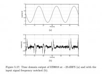
Also, the distortion residual you found has some similarity to the ES9018 I/V opamp output residual posted by Scott Wurcer. Scott said it was hump distortion. Attached below for reference.
Also, the distortion residual you found has some similarity to the ES9018 I/V opamp output residual posted by Scott Wurcer. Scott said it was hump distortion. Attached below for reference.
Attachments
The jury is still out on this... I need to build my own DAC I-V/filter circuit (work in progress for the ES9038q2m in Topping D10B) to verify how much of the effect actually is due to demodulation of RF glitches into variable DC offset, rather than just summed-up glitch energy as such... even with a blameless integrator/filter. The typical OpAmp I/V circuits we see for ESS DACs don't look like being blameless, with the OpAmp + its supply having to establish the full return path of any RF glitch/step energy.
Non-constant glitch energy piling up in the intergrator would be a baseline error that we cannot easily mitigate. Only way I could think of is massive paralleling of 8 or more channels with slightly different digital DC offset and/or common-mode dithering etc, to spread out and flatten the error. Probably an academic exercise, though....
Non-constant glitch energy piling up in the intergrator would be a baseline error that we cannot easily mitigate. Only way I could think of is massive paralleling of 8 or more channels with slightly different digital DC offset and/or common-mode dithering etc, to spread out and flatten the error. Probably an academic exercise, though....
No, so far I only played with the two ESS DACs (KTB and D10B) as is... which is async mode, running from local 100MHz crystal.@KSTR , Haven't read the whole thread yet, but assume if you tried disabling ASRC you found out that DPLL_BANDWIDTH has to be set to zero?
I have a third board which offers easy access to the I2C bus so could try different register settings with something like Ian Canada's ESS controller.
I'm aware of the findings presented by @bohrok2610 and others, like that glitch energy (and thus artifacts) scales directly with clock frequency, crystal vs. oscillator module may make a difference, and obviously reference voltage generation is paramamount, as is layout.
A long road.
Now that AKM 4490/93 are coming back, I admit I've lost interesst in ESS DACs as we will be using AKMs as originally planned in new products we are designing at work. Sometimes delays product development are a good thing, haha!
Used an Arduino myself for configuring ES9038Q2M registers. Have some early version code that works for reading and writing all the registers including the 16-bit and 32-bit register sets. Also have the basic initialization register settings. Happy to share if possibly useful. Changing the subject for a moment, also found that adding some differential input capacitance before the I/V opamps helped the sound. Used distributed filtering for that, a few inches of twisted pair wire-wrap wires close to the ground plane instead of a lumped cap.
Last edited:
The -20 dB error waveforms look quite familiar to me. I think I've seen waveforms like that when simulating low-order undithered sigma-delta modulators and subtracting a low-pass filtered version of the output signal from the input signal. Those were probably single bit modulators driven close to full scale, though.I would beg to differ. Looking at the time-domain residual is bascially looking at the sample value transfer function error directly, with only little deformation (at the top and bottom section of the exciting sine).
Only the observation of the development of the residual error vs level finally gave me the right clue what's really going on with the infamous "ESS hump"... a periodic ripple on top of the sample value transfer function. The total number of periods of that ripple correlated to the number levels of the final output DAC, bingo.
Staring at spectra doesn't give much insight, I would agree, though.
I was mixing up things, of course. It looks like folding distortion, or (equivalently) like the quantization error of an undithered multibit quantizer. No idea why you get a much attenuated quantization error of a rather coarse quantizer on top of the desired signal, though.

If the multibit sigma-delta modulator mainly switches between adjacent levels, maybe the transition density depends on the fractional part of the input signal?
If the multibit sigma-delta modulator mainly switches between adjacent levels, maybe the transition density depends on the fractional part of the input signal?
Last edited:
Marcel, ESS has touted their Hyperstream modulator as suppressing signal correlated noise in a unique way. There was a graphic showing a comparison between hyperstream verses competitor dac modulator noise as a function of DC offset level. Can't find that one right now, but do find one attached below. Might that make any sense with respect to your hypothesis?
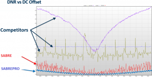
EDIT: Just found the other one 🙂
EDIT: Just found the other one 🙂
Attachments
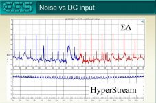
I don't know. Those noise plots show a periodicity of the noise with the input DC input level that ideally shouldn't be there, but the time average of the error would have to be periodic with the DC input level to get the distortion waveforms KSTR measured.
IME with similar implementation (PS, Vref, clocks, layout) ES9038Q2M has more high-order harmonics and phase noise than e.g. AK4490. THD compensation can be used for numbers game (lower THD+N) but is relatively useless for anything else as it is highly level/frequency/fs dependent. So I also switched my attention back to AKM dacs. First surprise was that the output stage I used on AK4490 with excellent results did not deliver at all with AK4493S.Now that AKM 4490/93 are coming back, I admit I've lost interesst in ESS DACs as we will be using AKMs as originally planned in new products we are designing at work. Sometimes delays product development are a good thing, haha!
Yeah, that's what I'm inclined to think as well. Varying transition density and thusly also varied glitch energy could be the key.If the multibit sigma-delta modulator mainly switches between adjacent levels, maybe the transition density depends on the fractional part of the input signal?
Besides that, I don't think the DWA has something to do with it directly as ESS claims to have taken care to avoid DC-induced limit cycles, but what do we know? ;-)
…Here's an example:
The circuit R1 D1 R2 has a gain of 1 if v(in)<0V and a gain of 0.5 if v(in)>0.6V, with a transition as the diode turns on. Its transfer function is on the left.
View attachment 1077156
Nice explanation, thank you, much appreciated (I was "lost" anyway in using two amps for the measures).
From the last graph shown (in blue) we then obtain the derivative of the transfer function and from this the function itself. Very effective. Considering that with the same level of signal y (red curve) the derivative does not assume the same value, we obtain two transfer curves: one for the increasing signal and one for the descending one. The reason is given by thermal effects, as you have already described, which introduces memory effects, not contemplated by the "static model".
I wonder how these aspects can be translated into a “black box” simulation model (only via Volterra kernels?) and after how they translate into effects on the perception of sounds for real devices. Have you made any attempts in this regard?
Last edited:
Not just that. It could simply be phase, that has to be corrected first, otherwise with enough phase shift your transfer function will look like a circle. Once this is done, there are indeed many differences between the "going up" and "going down" transfer functions. For example in a class AB amplifier, the two halves of the output stage use complimentary transistors, and these devices don't turn on and off at the same speed. So the crossover will look different depending on the polarity of the slew rate. If the circuit has problems, some part may be close enough to running out of current when slewing in one direction but not the other (a form of TIM). And... due to charge storage and other effects, the transfer function also depends on slew rate. Then there are thermal effects.Considering that with the same level of signal y (red curve) the derivative does not assume the same value, we obtain two transfer curves: one for the increasing signal and one for the descending one. The reason is given by thermal effects, as you have already described, which introduces memory effects, not contemplated by the "static model".
I didn't look into that. It was useful as a tool to sort output stage topologies though.I wonder how these aspects can be translated into a “black box” simulation model (only via Volterra kernels?) and after how they translate into effects on the perception of sounds for real devices. Have you made any attempts in this regard?
I didn't look into that. It was useful as a tool to sort output stage topologies though.
On this point I have developed both simulation models, static and dynamic.
For the static model I have done a lot of insights with the posts that I have already published (I have other in progress, such as the concatenation of systems and feedback). In summary, by injecting 2nd and 3rd harmonic distortions into musical signals, the listening effect (with blind tests) is what is commonly found: warm or dynamic expansion/compression. The least "fitting" aspect is that the distortion levels that I have to inject into the musical signals to hear changes are much higher than those resulting from measurements of real amplifiers: at least 1%, with 75-80dB SPL. A sign that the model is an “ideal” starting point, not taking into account the inevitable memory effects.
The dynamic model, much more complex, is based on Volterra's Diagonal Kernels. Simplifying as much as possible, here I measure the frequency trend of the distortion of each harmonic, in module and phase. Then, each Hi(f) curve is inserted into the model, according to the following classic scheme:
Last edited:

If it takes 1% added distortion to make something listenable, does that mean a live symphony performance is unlistenable?
Or maybe it means more along the lines of, something in the reproduction chain is so bad it takes 1% added distortion to mask it enough so that the system is listenable?
Or maybe it means more along the lines of, something in the reproduction chain is so bad it takes 1% added distortion to mask it enough so that the system is listenable?
I just meant that as 1 % of low-order distortion is barely noticeable, devices with a distortion of the order of 1 % can sound quite acceptable. Analogue tape recorders driven to 0 VU, for example.
Regarding how much distortion it takes before the distortion becomes audible, it can actually be quite small. I would remind people that I once sorted recordings of music playing through unity-gain audio opamp buffers in order of distortion by ear. It was in one of PMA's listening tests. PMA acknowledged that after he revealed which recordings were of which opamps, and the distortion measurements of each.
Moreover, I thought there was a little statistical evidence other people could almost do it too. One common mistake most made was to put them in reverse order. I think that was probably because sometimes a little very low level distortion can be mistaken for increased clarity. However, that type of mistake doesn't matter if the question is whether or not they sound different.
EDIT: I think the "1% to be noticeable" idea probably comes from the fact that it starts to sound more clearly like what people think of as distortion at that level. However, IME there are audible clues of lower than 1% distortion in a very clean system playing real music. IMHO its that low level IMD has a sound one can learn to recognize.
Last edited:
Without getting too off topic, I would briefly like to point out that most systems are full of insidious ground loops. Cleaning those up can make an easily audible difference in SQ and reproduction accuracy.
Also, it seems hard to understand how it makes sense to use a digital source to emulate distortion artifacts when that digital source is not of excellent quality. IMHO, something like a $500 dac is not up to task. I would have to test some of the best dacs in the world to find the one I thought most capable of accurately reproducing very small distortion artifacts. Steady-state AP measurements of a dac is no assurance it will be suitable for non-steady state test signal experiments. Sorry if that seems too blunt. Don't know how else to put it.
Also, it seems hard to understand how it makes sense to use a digital source to emulate distortion artifacts when that digital source is not of excellent quality. IMHO, something like a $500 dac is not up to task. I would have to test some of the best dacs in the world to find the one I thought most capable of accurately reproducing very small distortion artifacts. Steady-state AP measurements of a dac is no assurance it will be suitable for non-steady state test signal experiments. Sorry if that seems too blunt. Don't know how else to put it.
Last edited:
This is nice.Where applicable, it allows us both to study aspects that are difficult or impossible to obtain from direct measurements, and to predict the sound of specific distortion trends.
I'm going in a different direction, maybe simpler and more hands-on:
There are sonic differences between "low" THDs that should not be audible. This either means MarkW has superhuman ears, or the actual distortion is of a sort that's not well measured by the usual tests, and it is actually much higher and easier to hear, but it doesn't show up in the measurement results.
Of course the ultimate test would be input to output substraction. I'm gonna do that in my next project.
But I think we should look for ways distortion hides from the traditional FFT. I provided two examples above, one with a class AB output stage where the (real) distortion is much higher when the signal is not centered on zero (so a zero-centered THD test gives an unrealistically low number), and another with the power supply where increased distortion occurs only when the diodes are conducting, so it is averaged out by the FFT, and again seems much lower than it is. There must be others.
A live performance have zero distorsion for a person present, per definition.If it takes 1% added distortion to make something listenable, does that mean a live symphony performance is unlistenable?
......
//
- Home
- General Interest
- Everything Else
- How we perceive non-linear distortions