As Dissi has noted, this is not a new technique, but has been made more practical to implement in recent years.
I have used this method for the last 20 years, and have had the luxury of superb anechoic chambers in both the USA and Japan to be able to cross check the results.
There are some limitations to the accuracy, but they are small compared to the benefits of using the technique.
One limitation is the mathematics used to calculate diffraction are not totally accurate at the low frequencies, and the calculations are based on 2pi versus 4pi, not on nearfield versus farfield 4pi, so this limits the accuracy of the blend region.
I don't ever remember seeing a paper showing calculated versus measured to good accuracy. If anyone knows of one, please let me know! Otherwise it is on my list to do, just haven't had the time to do it.
One thing you should watch for when you blend is that you have the correct phase response matching, otherwise although the amplitude will blend, the phase will not.
Andrew
Hi Andrew,
Jeff was assuming that you would splice curves first, then Hilbert transform the resultant for phase. Otherwise, for measurements including phase, I assume you would add delay until your nearfield curve (for low frequencies) matched the phase of your 1 or 2 meter curve (presumably with air path pulled out). You would have to Hilbert transform the 4pi/2pi shelf as well, since it would contribute some phase wiggles.
A bit messy but not everyone has "the luxury of superb anechoic chambers".
Cheers,
David
Hi Dave.
Yes, the point I was making was that I had great chambers where I was able to assess the various methods of measuring, and determine where the errors creep in. I don't have my own one in Southern California any longer, so I do rely more on the splicing technique, though I do back that up with calculations from the impedance curve, in-box and acceleration measurements to make sure my results correlate well with all the methods, and custom BEM to calculate the diffraction, then a final check periodically in the chamber in Japan.
You shouldn't have to do a Hilbert transform on the shelf response as long as it is original calculated with phase information.
I agree that these methods are "messy". They take a long time to do if you want good accuracy, but with modern CAD Xover design you only have to do them once, so it's worth doing well.
One thing to be aware of, is that even a good chamber is not totally accurate and needs a correction curve applying at low frequencies. Unfortunately, this correction curve varies with speaker and microphone placement, so with a rear vent on a reflex system it is impossible to get a fully accurate summation, since the vent and driver would need different correction curves. Therefore I have to resort to measuring the speaker as a closed box, then applying the calculated difference curve between closed box and vented box response.
Andrew
Hi Dave.
Yes, the point I was making was that I had great chambers where I was able to assess the various methods of measuring, and determine where the errors creep in. I don't have my own one in Southern California any longer, so I do rely more on the splicing technique, though I do back that up with calculations from the impedance curve, in-box and acceleration measurements to make sure my results correlate well with all the methods, and custom BEM to calculate the diffraction, then a final check periodically in the chamber in Japan.
You shouldn't have to do a Hilbert transform on the shelf response as long as it is original calculated with phase information.
I agree that these methods are "messy". They take a long time to do if you want good accuracy, but with modern CAD Xover design you only have to do them once, so it's worth doing well.
One thing to be aware of, is that even a good chamber is not totally accurate and needs a correction curve applying at low frequencies. Unfortunately, this correction curve varies with speaker and microphone placement, so with a rear vent on a reflex system it is impossible to get a fully accurate summation, since the vent and driver would need different correction curves. Therefore I have to resort to measuring the speaker as a closed box, then applying the calculated difference curve between closed box and vented box response.
Andrew
Hello Andrew,
I wrote the paper mainly for the home DIY'er, for whom this method may be new because it differs from the hard splice that is detailed in "Testing Loudspeakers" by Joe D., and what is shown in a lot of measurement software instructions. To further complicate things Stereophile shows a rather messed up splice that always artificially elevates the data below 200Hz. I appreciate the fact that others have known of it for quite some time, it just wasn't very mainstream.
Since it was mainly targeting DIY'ers, many of whom use my Passive Crossover Designer, we made it easier and eliminated "splicing" the phase response and just extract the minimum phase from the final blended response at the end. This will work well in my program which uses entered physical offsets for driver locations. (I have another paper the details how to determine exactly what those offsets really are.) It's pretty accurate through the crossover range, as the final summed response will match the simulation very nicely.
Diffraction calculation at lower frequencies is still a bit hard to get right, because, as you pointed out, all acoustic spaces influence the low-end response in some way, even anechoic chambers, so it's hard get this just right. My diffraction model is based on the Vanderkooy model and has proven to be very accurate. We had this validated for us a few years ago with work done in an anechoic chamber, but that's a story for another time.
There is, however, some new math on low frequency diffraction modeling that you may be interested in. It is in a article written by Jeff Candy titled "Accurate Calculation of Radiation and Diffraction from Loudspeaker Enclosures at Low Frequency". It can be found in JAES January, 2013 edition. Jeff addresses the effect that radiation has on diffraction, especially in the transition from 2 Pi to 4 Pi region. If you haven't noticed it, you might take a look.
Jeff B.
Hi Jeff. Yes, I realize your motivation for the DIY'er, and appreciate your efforts to bring this to their attention. I am a bit (a lot!) of a pedant when it comes to accurate measuring of speakers, hence my commentary. I see so many examples of measurements where it is clear that the curves show as much about the inaccuracy of the measurement technique applied as they do about the performance of the device under test!
I'm interested to hear that you did valuation of your diffraction model vs measurement, but I still want to do my own")
As for the Vanderkooy technique, he had told me long ago that the inaccuracies were mostly at low frequencies, which is what I based my comments on.
Thanks for the info on the Candy paper. If I have in fact read it, I have forgotten, so I will re-read it.
I do remember long ago, while I was at KEF, that we had a French student that had done a project on diffraction, by measuring the effect of different driver sizes upon differing box sizes, and found a very simple algorithm that would give a close fit based on just a few parameters, but I no longer have a copy of the paper that she wrote for us.
Andrew
I'm interested to hear that you did valuation of your diffraction model vs measurement, but I still want to do my own
As for the Vanderkooy technique, he had told me long ago that the inaccuracies were mostly at low frequencies, which is what I based my comments on.
Thanks for the info on the Candy paper. If I have in fact read it, I have forgotten, so I will re-read it.
I do remember long ago, while I was at KEF, that we had a French student that had done a project on diffraction, by measuring the effect of different driver sizes upon differing box sizes, and found a very simple algorithm that would give a close fit based on just a few parameters, but I no longer have a copy of the paper that she wrote for us.
Andrew
Hi Jeff.
Just downloaded the paper and read it. The math is beyond me.......but the results are interesting. It confirms my suspicions about the limits in accuracy of the BEM techniques, and also the variability of the nearfield response, although this is mainly in level at low frequencies.
I had in fact noticed this long ago, that the supposed leveling off of nearfield pressure change as one approaches the driver only applies for a flat piston in 2pi. For a cone this does not happen, and for a cone in a box in 4pi it does not happen, and for the vent it certainly never happens. For the latter reason, the technique of measuring a vented box response by adding vent and cone response adjusted according to their respective radiating areas is extremely inaccurate. In fact, a much better method is simply to measure just the vent and double differentiate the response. The reasoning is crafty but elegant
Andrew
Hi Andrew.Just downloaded the paper and read it.
Yes, its unfortunate that some aspects of the paper are far from transparent. The method in practice also has some convergence subtleties that require care in application. Despite that you seem to have gleaned the implications of a number of the results. Let me emphasize that a good deal of the results are not new but were of course known earlier. For example, that nearfield measurements are not diffraction-free at all wavelengths was discovered (or at least documented) first by Vanderkooy. So really I just used the method to corroborate these earlier results and extend them a bit to more realistic geometry.
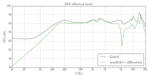
In the context of the present discussion, it might be useful to illustrate the typical sort of "incorrect" reconstruction to be expected from methods which have significant low-frequency error. So, below I show a few plots which illustrate how reconstructions differ when using (1) the MFS method and (2) the DED method (which is a more recent high-frequency approach by Urban, et al, JAES 52 (2004) 1043).
This is an easy example -- its a small full-range speaker (the Zaph Hi-Vi B3S single driver system) so the room is effectively "large". The microphone was closer than 1m so the level is slightly higher than the true SPL at 2.83V/1m.
- The first plot shows the quality of overlap between (a) the nearfield+diffraction data and (b) gated farfield for the DED model. The overlap seems good from about 500Hz to 1kHz. The nearfield level was adjusted to match the farfield, on average, from 400-800Hz.
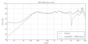
- The second plot shows the same overlap test for the MFS method (which is accurate down to 0Hz). Now the agreement is good from about 120Hz to 2kHz. Much better.
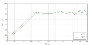
- The third plot shows the bottom line; namely, the final reconstructions of the anechoic response. Here we find the DED method underestimates the response everywhere below about 500Hz. Indeed, if you look at Zaph's reconstructed response, you see the flatness below 500Hz characteristic of the DED method, not the peak at 150Hz seen in MFS.
Attachments
Hi Jeff.
Thanks for the response. My comments about your paper were not to imply a lack of transparency on your part, simply a lack of mathematical dexterity on my part! The rest of the paper is fine. It just reminds me studying for my Physics degree at University. The Quantum Mechanics lecturer at the time broke down after repeated requests to explain the subject, and declared "I'm sorry......I .. just ...can't come down to your level!!"
I may not remember much now about quantum mechanics, but I do remember that comment.
Your results are very informative, and show the difficulties involved in truly assessing low frequency response. They at least show that even for a small system, the gated farfield response contains significant errors!
thanks
Andrew
A very interesting paper. I have been using something similar for years.
What I do instead of a baffle step model, is to use a spherical enclosure model which is adjusted to the near field data, just as the paper describes, but usually using more than just one point (just in case that point has some problems). The spherical model will have all the correct diffraction up to the point where the sphere is about the same size as the wavelength. At that point the two will begin to differ (neither being very accurate actually). But if the sphere, or cabinet, is not too large then there is no problem as this would be fairly high in frequency. A very large cabinet with a small speaker might be an issue, but this isn't very common.
The two curve are then blended, just as described in the write-up. I used to use point matching but quickly learned that this didn't work very well.
PS. I taught physics to undergrad non-science majors (no calculus) and I gave up after a few years because it is just not possible to teach the subject with no math. When I think of physics I see the math. I don't know how to see it any other way.
Last edited:
A very interesting paper. I have been using something similar for years.
What I do instead of a baffle step model, is to use a spherical enclosure model which is adjusted to the near field data, just as the paper describes, but usually using more than just one point (just in case that point has some problems). The spherical model will have all the correct diffraction up to the point where the sphere is about the same size as the wavelength. At that point the two will begin to differ (neither being very accurate actually). But if the sphere, or cabinet, is not too large then there is no problem as this would be fairly high in frequency. A very large cabinet with a small speaker might be an issue, but this isn't very common.
Earl,
Thinking of Olson's study of diffraction from loudspeaker cabinets of different shapes and sizes, the "spherical model" would seem to be an overly general representation of the diffraction response since it is essentially a smooth monotonic transition. Boxy loudspeakers (e.g. "cube" in Olson's figure) have a more oscillatory approach to the high frequency regime. Figure provided below for reference.
Does your approach capture the oscillations for a rectangular box, and if so can you elaborate?
-Charlie

Thread link: http://www.diyaudio.com/forums/multi-way/196668-diffraction.html
It would not capture the oscillations the same way as a box, that what I was saying. But if you look at your own data you will see that you don't even get to the oscillations portion of your model. In the region that counts the two should be very similar. Even in Olsen's data below 300 Hz they are all pretty much the same.
I should also mentioned that Olsen is not a good source because a lot of what he published has not turned out to be correct. If you look through texts showing a spherical model (including mine) you will see that a spherical model does have ripples. Why Olson's doesn't is a mystery. It looks like his source is very small, or his sphere is very large, or the drawing is completely wrong.
If I get the chance I will show a spherical model for a typical sized system.
7/8" diameter driver diaphragm, 24" diameter sphere.It looks like his source is very small, or his sphere is very large, or the drawing is completely wrong.
If I recall correctly, Olson actually made these curves by mounting a microphone rather than a speaker in the shapes of interest. He then measured a second speaker twice, once with the test object on the mic and once without it, and plotted the differences.
Same difference in the end, but an interesting approach.
David
Same difference in the end, but an interesting approach.
David
Here is a plot of the diffraction gain computed for a point source on a sphere of diameter 24" (radius=30cm) measured at a distance of 2m from the point source along the axis of the point source. The result agrees pretty well with Olson. The calculation method is straightforward eigenfunction expansion (using 90 Legendre harmonics). The gain here misses the very large primary (and secondary) peaks and dips of the rectangular enclosure.A speaker that small and a sphere that big would not show much ripple. A larger speaker or smaller sphere would.
Attachments
I still believe that those peaks are out of band. Could you plot both on the same plot using something more comparable like a sphere of the same volume as the enclosure with a driver size more like a real driver. I am willing to bet that below 500 Hz the two will not differ by more than one dB. In my work I fit between 200-300 Hz, sometimes as high as 400 Hz, never 500 Hz.
Here is a plot of the diffraction gain computed for a point source on a sphere of diameter 24" (radius=30cm) measured at a distance of 2m from the point source along the axis of the point source. The result agrees pretty well with Olson. The calculation method is straightforward eigenfunction expansion (using 90 Legendre harmonics). The gain here misses the very large primary (and secondary) peaks and dips of the rectangular enclosure.
That would be my concern - the primary baffle peak above the step frequency. Since we all tend to use rectilinear boxes we will almost always have to deal with some significant baffle diffraction peaking at the top of the 4Pi - 2Pi transition. This peak contributes to, and extends the step in amplitude. And its presence is part of what I am using to align the near-field and far-field response data with.
I recognize the potential errors in my model at lower frequencies, but there is a point where near-field data is full blended and that is controlling the level, not the diffraction model. What I need is reasonable accuracy in the 150 - 1200 Hz range to establish the correct alignment for blending the data.
Jeff
- Status
- This old topic is closed. If you want to reopen this topic, contact a moderator using the "Report Post" button.
- Home
- Loudspeakers
- Multi-Way
- Nearfield/Farfield curve splicing