On fitting characteristic curves.
I finally got around to do a pedestrian version of measuring (Vgs, Vds, Id) tuples to characterise a given device.
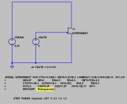
I use a lab power supply connected to gate and drain of the jfet.
Between gate and source I put in various fixed resistors and measure the voltage dropped.
Vds = Vdg + Vgs and Id = Vgs / Rsource (or measure it directly)
With Vgd = 2 .. 10V and Rsource = 0 .. 1kOhm I cover Vgs from 0 close to -0.6V.
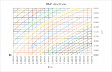
I can then fit the regular Id=beta*(1+lambda*Vds)*(Vgs-VTO)^2 by minimising the RMS differences between modelled and measured Id values.
What I want to share here is that the RMS difference minimum is very shallow along a step trough when you plot it along VTO and beta. The attached graph shows “iso RMS” lines (and some Excel artefacts) and you can see that you can vary VTO within a range on the order of 100mV and get a fit of almost equal quality if you adjust beta accordingly.
So much for reproducing fitted VTO values in measurements. You can basically pick a number for VTO (eg. Vp @ 1% Idss) and use beta for fitting. The quality of your model (in a range of Vgs = 0 .. -0.6mV and Vds = 2V .. 10V) will only be mildly affected.
The story will be different if you are interested in a different operating region.
I finally got around to do a pedestrian version of measuring (Vgs, Vds, Id) tuples to characterise a given device.
I use a lab power supply connected to gate and drain of the jfet.
Between gate and source I put in various fixed resistors and measure the voltage dropped.
Vds = Vdg + Vgs and Id = Vgs / Rsource (or measure it directly)
With Vgd = 2 .. 10V and Rsource = 0 .. 1kOhm I cover Vgs from 0 close to -0.6V.
I can then fit the regular Id=beta*(1+lambda*Vds)*(Vgs-VTO)^2 by minimising the RMS differences between modelled and measured Id values.
What I want to share here is that the RMS difference minimum is very shallow along a step trough when you plot it along VTO and beta. The attached graph shows “iso RMS” lines (and some Excel artefacts) and you can see that you can vary VTO within a range on the order of 100mV and get a fit of almost equal quality if you adjust beta accordingly.
So much for reproducing fitted VTO values in measurements. You can basically pick a number for VTO (eg. Vp @ 1% Idss) and use beta for fitting. The quality of your model (in a range of Vgs = 0 .. -0.6mV and Vds = 2V .. 10V) will only be mildly affected.
The story will be different if you are interested in a different operating region.
Attachments
Yep, to disambiguate between VTO and BETA you need to give higher weight to the linear region (VDS < 0.8).
Another option is: you can boldly declare, "I don't care about the linear region! My circuits will always operate the JFET where it is an excellent voltage controlled current source!"
The second candidate is especially appealing if your simulator doesn't provide Taki-equation models.
Another option is: you can boldly declare, "I don't care about the linear region! My circuits will always operate the JFET where it is an excellent voltage controlled current source!"
The second candidate is especially appealing if your simulator doesn't provide Taki-equation models.
Last edited:
Well, bold or not so bold that is my current objective.
I am looking at circuits where I want the jfets in saturation and I want to simulate the devices I own (as opposed to 99% of the devices in the universe).
And my simulator apparently doesn't do so well in the linear region.
Does yours?
I am looking at circuits where I want the jfets in saturation and I want to simulate the devices I own (as opposed to 99% of the devices in the universe).
And my simulator apparently doesn't do so well in the linear region.
Does yours?
@Mark -- what program are you using for optimization? I use the Excel Solver to minimize the squared error, or log-squashed error.
I used the optimizer in Python, you can specify any weighting you want as a function passed to the optimizer. The problem is what do you want? None of these results will model open-loop distortion in a simple circuit particularly well. For instance the second harmonic null trick used by Schoeps in their microphone's phase splitter does not simulate at all.
What I want to share here is that the RMS difference minimum is very shallow along a step trough when you plot it along VTO and beta. The attached graph shows “iso RMS” lines (and some Excel artefacts) and you can see that you can vary VTO within a range on the order of 100mV and get a fit of almost equal quality if you adjust beta accordingly.
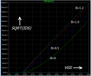
But the transconductance (hence gain) is a function of only beta and Id and I would think this is at least one thing you would want to get as close as possible. Using the value of Vto from the extrapolated slope of sqrt(Id) vs Vgs, taking care to get the portion of it closest to a straight line, will help you get the best fit to actual gain vs Id. If you're forced to use the basic model I would choose this. If you use LTSPICE you then can also correct for the slope not being 1/2. IIRC you might need the paper they reference in the users manual to compute B from the slope. Mark has a copy if he has the DVD collection. If it's one of the things they don't archive I have it.
Jackinnj, generally I use a simulated annealing subroutine I wrote in the 90s, closely following the algorithm described in Corana et al, ACM Transactions on Mathematical Software, 1987 (link to pdf). Occasionally I use the Solver too, same as you. Simulated annealing is compute intensive, to be sure. But CPUs are fast and cheap these days. I don't mind waiting a bit longer in exchange for the peace of mind that SA finds the global optimum; it doesn't get trapped in local minima.
Scott,
Fitting a straight line to sqrt(Id) instead of fitting a parabola to Id basically amounts to giving higher weights to smaller Id values, doesn't it?
Or do you suggest this procedure to censor the data to give most relevant results?
If anyone could provide me with that paper (A. E. Parker and D. J. Skellern, An Improved FET Model for Computer Simulators, IEEE Trans CAD, vol. 9, no. 5, pp. 551-553, May 1990) I'd be grateful, b/c I would like to understand what LTSPICE really does.
The present fitting problem is so simple (cf. my pic above) you can use any solver.
The problem is what do you want?
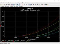
Eureka! If the JFET is going to be used in a cascode @ VDS = 4.0 volts, then what I actually want is Ids vs. Vgs @ VDS=4.0 volts. I don't care about other VDS values since the circuit won't operate there.
So: take 3 datasets on the curve tracer: (i) Id-Vg @ VDS=3.5 volts; (ii) Id-Vg @ VDS=4.0 volts; (iii) Id-VG @ VDS=10 volts {to get the output conductance parameter LAMBDA}. Sweet!
Just remember to only use this model for 4V cascodes and nothing else!
I have an IDSS histogram, yes, but I won't be uploading it to diyAudio, no.
If you desire to see a histogram very urgently, you had better hurry, mouser.com says the BF862 is "end of life". They still have 20K parts to sell, at a fairly low price: (link). Buy a few hundred to own and to use and to hoard; possibly reselling the excess in a few years, at greatly inflated prices.
You will probably want a socket to make testing these little SMD babies less cumbersome. I bought (these from eBay). They are SOT23-6pin which the BF862 fits nicely. The SOT23-3 is mechanically compatible with the SOT23-6. I also bought (this considerably more expensive socket) from Peak, the people who sell the battery powered, hand held curve tracer "Atlas DCA75".

- Home
- Amplifiers
- Solid State
- LTSPICE models of worst-case BF862 JFETs