wikipedia wrote:
Oh yes, I recognize the red logo. Sounds good.illy is a brand of coffee produced in Trieste, Italy. illy produces only one blend in three roast variations: normal, dark roast or decaffeinated. The blend is packaged as beans (yet to be ground), pre-ground coffee or E.S.E. pods.
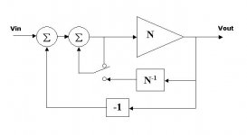
What a trip! Got your towel with you?Well, see, I have these two black boxes (one for each switch postion) built with the same forward path amp block, having identical transfer functions, and being told that yet they have different loop gains.
No.
Again, in this case, I can built two black boxes, one for each switch position. By your own account, these boxes have identical transfer functions. They are built with the same forward amp blocks. You cannot come up with any transfer function measurement that identifies which is which. Yet you tell me you measure different loop gains. How can that be?
Jan Didden
I know what you are asking. But let's just decide how to measure loop gain first.
This diagram shows a feedback loop around an arbitrary gain function "?". Do you agree or disagree that the loop gain can be measured at A, B or C and that all three measurements will be the same?
This diagram shows a feedback loop around an arbitrary gain function "?". Do you agree or disagree that the loop gain can be measured at A, B or C and that all three measurements will be the same?
Attachments
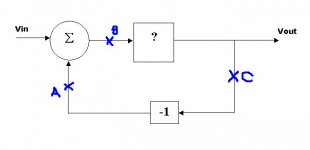
traderbam said:By "arbitrary gain function" I mean to say that "?" could contain any network of gains and PFB and NFB loops and summers.
No. Only if '?' would contain no feedback network elements (pos or neg or any combination) would I agree that A, B, C would give the same loop gain. As soon as '?' is in any way recursive, it doesn't anymore.
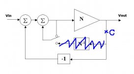
I think we lose again focus. I agree that the particular case you showed before with the two summers in series and the isolated pfb loop at the input of N looks innocent enough to say, OK, we measure loop gain at C and that's it.
But we can't just ignore the fact that those two black boxes I made from that last circuit give me two different loop gain values at C for essentially the same circuit. We need to resolve that. Once we do, we can apply that to H.EC and make meaningfull comments. As long as measurements on the same circuit give inconsistent results, you cannot make meaningfull comments based on those measurements. We have to resolve that.
Jan Didden
Jan wrote:
Herein lies the cause of our discord. I cannot think of any content of "?" that would make the LOOP gain any different at A, B or C. That's because the loop gain is calculated by multiplying the transfer functions together of each block in the entire loop, so changing from A to B to C just multiplies the same blocks in a different order. Since the result does not depend on the order of multiplication (a*b*c = b*c*a = c*a*b) surely it cannot matter at which point the LOOP gain is calculated or measured? Can you help me understand where I have gone wrong?No. Only if '?' would contain no feedback network elements (pos or neg or any combination) would I agree that A, B, C would give the same loop gain. As soon as '?' is in any way recursive, it doesn't anymore.
I have no problem with two circuits having the same Vout/Vin (external transfer function) whilst having different LOOP gain measurements at C. Why should the measurement at C be the same?But we can't just ignore the fact that those two black boxes I made from that last circuit give me two different loop gain values at C for essentially the same circuit. We need to resolve that. Once we do, we can apply that to H.EC and make meaningfull comments. As long as measurements on the same circuit give inconsistent results, you cannot make meaningfull comments based on those measurements. We have to resolve that.
traderbam said:Jan wrote:
Herein lies the cause of our discord. I cannot think of any content of "?" that would make the LOOP gain any different at A, B or C. That's because the loop gain is calculated by multiplying the transfer functions together of each block in the entire loop, so changing from A to B to C just multiplies the same blocks in a different order. Since the result does not depend on the order of multiplication (a*b*c = b*c*a = c*a*b) surely it cannot matter at which point the LOOP gain is calculated or measured? Can you help me understand where I have gone wrong?[snip]
I don't have all the answers, otherwise I wouldn't bother with this forum
")
In your particular example here, for instance, what would be the transfer function of the pfb block looping back into itself? Since its Vout would be its Vin + its Vout again, we get Vin is zero. A meaningless result. However, if you properly re-shuffle those loops (without changing the functionality) as we've been doing, you DO get a meaningfull result for *the* loop gain.
traderbam said:[snip]I have no problem with two circuits having the same Vout/Vin (external transfer function) whilst having different LOOP gain measurements at C. Why should the measurement at C be the same?
Well, you've got to be kidding here! We've done the exercise with the SPDT switch leading to two identical circuits (functionally) having at C two different loop gain measurements. Since it is loop gain that determines the transfer function, that in itself should ring a bell large enough to park your car in.
Nothing is stopping me from making a switch with an infinite number of positions, making an infinite number of identical circuits by shuffling around the feedback loops. That would lead to an infinite number of different loop gains at C, all with the same transfer function. That would pretty much make any loop gain measurement irrelevant.
Jan Didden
Aha. Jan my friend, what makes you think that the transfer function (Vout/Vin) is determined by the LOOP gain at C?Since it is loop gain that determines the transfer function, that in itself should ring a bell large enough to park your car in.
This may shed some light on it. From the guy that does the spice developments for Beige Bag:
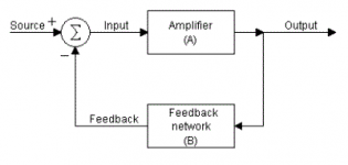
Before getting into the simulation loop gain methods, it is important to remember that most of the college and academic discussions concerning loop gains, and servos in general, are based on a BLOCK DIAGRAM model representation. See Figure 1, from Reference 1.
Figure 1
Typical Block Diagram
Each block in a BLOCK DIAGRAM has the following characteristics:
1. It is infinite impedance at its input (if it represents a voltage-to-whatever transfer function. If it represents a current-to-whatever transfer function the input impedance is zero.)
2. It has effectively zero output impedance (if it represents a whatever-to-voltage transfer function. If it represents a whatever-to-current transfer function the output impedance is infinite.)
3. The signal flow is unidirectional. Changes at the output of a block due to loading or signal application do not create changes at the input of a block due to direct transmission through the block in the reverse direction. Information flows only in the direction of the arrows.
Note in particular point 3. When you leave the pfb block in-line, so to say, and don't cut that part of the loop, you violate characteristic 3.
I don't know WHY that characteristic is a condition, but it does lead to different loop gains at C for the same circuit. Once you include the pfb block in the loop-cut thing, i.e. make all the arrows go in the same direction, those differences disappear.
Block diagram attached.
Jan Didden
Attachments
traderbam said:
Aha. Jan my friend, what makes you think that the transfer function (Vout/Vin) is determined by the LOOP gain at C?
This is my reasoning: Why do you measure loop gain? To get information about the transfer function, isn't it? Gain, stability, phase margin, etc. So if you can get pretty much any loop gain measurement result for a certain circuit if you insist on measuring it always at C, no matter what the block diagram, as we have seen, what is then the relevance of the loop gain measurement?
If you have a circuit with a certain phase margin, you would want to see that same phase margin in that circuit even if you would rearrange it's blockdiagram without changing its transfer function, no? And by insisting to measure it always at C (that is, always at the point where the nfb branch of the multi-loop fb system connects to Vout), you can get pretty much any phase marging measurement you want, even with identical circuits.
Jan Didden
No. It's to get information about the gain and phase of the feedback loop.This is my reasoning: Why do you measure loop gain? To get information about the transfer function, isn't it?
Because it tells you how stable the equivalent real circuit may be for each block diagram.Gain, stability, phase margin, etc. So if you can get pretty much any loop gain measurement result for a certain circuit if you insist on measuring it always at C, no matter what the block diagram, as we have seen, what is then the relevance of the loop gain measurement?
Not necessarily, no.If you have a circuit with a certain phase margin, you would want to see that same phase margin in that circuit even if you would rearrange it's blockdiagram without changing its transfer function, no?
You can get different feedback gains and phase margins for different circuits that have similar Vout/Vo. I'm not sure you can get whatever you want.And by insisting to measure it always at C (that is, always at the point where the nfb branch of the multi-loop fb system connects to Vout), you can get pretty much any phase marging measurement you want, even with identical circuits.
This is why when you implement a HEC topology into a real circuit you make a high NFB loop too. You can measure it in simulation at point C and you can measure it on the bench at point C. You deny it at your peril because having lots of NFB in the circuit (regardless of how the gain was generated) can be a real stability problem. In a mathmatical block diagram you don't see the side-effects of high NFB that you will see in a real circuit (if you are lucky you will - and you will certainly hear them).
Jan, regarding those block diagram rules. They are normal assumptions for all block diagrams and they apply to ours. These rules do not apply to calculating loop gain of a circuit...provided the calculation or simulation includes the interface impedances then all is valid.
To make more sense of the PFB you can put the 'a' factor back into the loop and then calculate the loop gain. You get a limiting case where the feedback approaches infinity as 'a' approaches 1.
To make more sense of the PFB you can put the 'a' factor back into the loop and then calculate the loop gain. You get a limiting case where the feedback approaches infinity as 'a' approaches 1.
Some summary views on EC
There are at least three valid ways of looking at Hawksford Error Correction (HEC).
The first view of HEC is the error correction view. Here the error produced by the output stage is measured and “replaced” at the input. In the case of an emitter follower output stage, the gain of the emitter follower is slightly less than unity. The way in which it departs from unity accounts for its distortion. The error correction seeks to restore the gain to exactly unity by adding the signal shortfall back to the input.
To illustrate, assume that the gain is 0.95 and the signal level is nominally 10 V at the output. This means that 10.53 V must be at the input to the emitter follower output stage. The 0.53 V of loss or “error” is measured as such and then added to the original input of the system, so that the actual input only needs to be 10 V. Seen this way, the 0.53 V error is being exactly corrected. This is what gives rise to the use of the term “error correction” in describing this approach. If the amount added back is too large or too small, the correction will not be perfect, and this gives rise to the null seen as adjustment is made.
This view of the HEC architecture is completely legitimate, but there are caveats. Stability of the arrangement must be maintained, and in practice this is straightforward. As with any “cancellation” technique, phase and amplitude must be exact. In practice, this will not be the case, especially due to the phase error caused by the necessary compensation. The “correction” null will thus not be perfect, but will get extremely deep as frequency goes down in comparison to the compensation rolloff frequency of the EC loop.
The error correction view of HEC is like the dual of more conventional feedforward error correction. Indeed, if the measured error of the output stage is fed forward (instead of fed back) and summed with the output, the same distortion reduction and distortion spectrum will result as with HEC if the error measuring bandwidth is the same.
The second way of looking at HEC is the negative feedback view. Here the HEC arrangement is seen as one including both a positive feedback loop in front of the output stage and a negative feedback loop around the output stage. The positive feedback loop has unity positive feedback, so that it produces a local stage gain of infinity. Thus, the unity gain negative feedback loop then placed around the output stage has a loop gain of infinity and thus error is driven to zero in conventional negative feedback fashion.
As a negative feedback system, this arrangement needs some form of compensation so that the loop gain of the outer NFB loop rolls off in a controlled way. That compensation will tend to cause the positive feedback factor to decrease below unity at high frequencies, resulting in lower gain from the positive feedback stage and thus less error reduction. Behavior will be the same as in the first view above, with very high amounts of error reduction available at frequencies that are low compared to the compensation rolloff frequency.
In principle the unity gain positive feedback loop in this view could be replaced with a large lump of gain with an appropriate rolloff. However, in practice it might be difficult to achieve the same level of performance with a conventional lump of gain, and complexity would likely increase.
The negative feedback view of HEC readily allows one to break the outer NFB loop and assess the loop gain characteristic for stability. One will generally see that the loop gain rolls off at 6 dB per octave over several decades as a result of the effect of the compensation gain and phase on the inner loop’s positive feedback factor. The feedback factor might start at 100 dB at 100 Hz and fall though 0 dB at 10 MHz at 6 dB per octave. Note, however, that in a real circuit, the 100 dB number at LF implies a trimmed gain accuracy to 0.001%.
The third view of HEC is the “low feedback” view. Here it is recognized that the emitter follower output stage needs a little bit of a gain boost to get its gain back to exactly unity. This can only be accomplished with a very slight bit of net positive feedback. 1/(1-AB) factor will have to come out to about 1.053 in this case. The amount of slight positive feedback is arrived at by what amounts to a bridge circuit, where a subtraction takes place between what is put into the output stage and what comes out of the output stage. This creates a very small residual amount of feedback that has a very small amount of loop gain that can be positive or negative feedback. In this case, it will usually be slightly positive as mentioned above.
The magic in this view of HEC is that the feedback factor is adaptive in that the error in the output stage adapts, or adjust the small amount of feedback needed to correct the incremental gain of the stage. The key here is to realize that the actual amount of correction that needs to be applied to the emitter follower output stage is quite small, so that only a very small amount of net feedback is necessary.
The important point is that all three of these ways of looking at HEC are valid. Each offers its own insights, and each has its limitations in what it reveals. The error correction view can be very intuitive for some, but it does not excel at revealing stability issues. The negative feedback view is probably better at revealing stability issues in a traditional feedback analysis sense, but it can be confusing to some because of its implied positive feedback and infinite gain.
Cheers,
Bob
Hi Bob,
Great summary of the 3 main approaches that have been debated ad nauseum in the many pages of this thread.
 My opinion, for what it is worth
  (note the falling $ exchange rate), is that although these three approaches may be valid in the sense that it is valid for people to hold different views, I believe two of the three are misleading because they contain false premises. Does this matter? Yes, because when a conceptual view contains bad assumptions it usually causes disappointment at the implementation stage.
 It is mathematically impossible. Your example side-steps this.


But it isn’t just as I see it. The fact is that if you or anyone else measure the NFB in a real circuit or any simulation or calculate it on paper it exists. And in no small measure. And just like any other NFB system the NFB loop gain is there all the time, it doesn’t disappear when the output error is zero.
This is not just another way to “view” it…it is always a high NFB system.
My concern is for others who may be undertaking this form of distortion reduction if they are led to believe that there is negligible NFB involved…they could easily overlook stability issues. Especially if the reduction in phase margin and the increase in forward distortion that occurs as the circuit is tweaked towards its so-called “null” condition is not recognized.

Brian
Great summary of the 3 main approaches that have been debated ad nauseum in the many pages of this thread.
Predictably, I have to beg to differ, if that’s ok.The important point is that all three of these ways of looking at HEC are valid.
My opinion, for what it is worth (note the falling $ exchange rate), is that although these three approaches may be valid in the sense that it is valid for people to hold different views, I believe two of the three are misleading because they contain false premises. Does this matter? Yes, because when a conceptual view contains bad assumptions it usually causes disappointment at the implementation stage.The false premise is the “feed-forward in reverse” notion: applying some signal at the input that exactly corrects the output error, derived from the output. I maintain it is impossible to ADD a linear function of the output signal of a non-linear amp back to its input and cancel its output error.The first view of HEC is the error correction view.
It is mathematically impossible. Your example side-steps this.The false premises here are (1) that the requirement of a small voltage correction at the input to the output stage implies that only a small amount of feedback gain is required and (2) that this small amount of feedback is proportional in some way to the size of the output error. Neither of these assertions makes any sense to me at all. Just because the signal at the output device input needs a small voltage correction does not imply that the feedback required is small too. I dislike this “view” because it re-enforces the conceit that HEC does not require high NFB to work.The third view of HEC is the “low feedback” view.
This is reality as I see it.The second way of looking at HEC is the negative feedback view.
But it isn’t just as I see it. The fact is that if you or anyone else measure the NFB in a real circuit or any simulation or calculate it on paper it exists. And in no small measure. And just like any other NFB system the NFB loop gain is there all the time, it doesn’t disappear when the output error is zero.
This is not just another way to “view” it…it is always a high NFB system.
My concern is for others who may be undertaking this form of distortion reduction if they are led to believe that there is negligible NFB involved…they could easily overlook stability issues. Especially if the reduction in phase margin and the increase in forward distortion that occurs as the circuit is tweaked towards its so-called “null” condition is not recognized.
This is the only thing I find novel or interesting about HEC. The use of a synthetic gain block in place of a device gain without PFB. And this is really interesting and worth considering in any circuit where gain is required. There is a non-trivial trade-off to be made between gain and phase margin and distortion and output impedance. I’d like to explore this further.In principle the unity gain positive feedback loop in this view could be replaced with a large lump of gain with an appropriate rolloff. However, in practice it might be difficult to achieve the same level of performance with a conventional lump of gain, and complexity would likely increase.
Brian
traderbam said:Hi Bob,
Great summary of the 3 main approaches that have been debated ad nauseum in the many pages of this thread.
Predictably, I have to beg to differ, if that’s ok.
The false premise is the “feed-forward in reverse” notion: applying some signal at the input that exactly corrects the output error, derived from the output. I maintain it is impossible to ADD a linear function of the output signal of a non-linear amp back to its input and cancel its output error.
The false premises here are (1) that the requirement of a small voltage correction at the input to the output stage implies that only a small amount of feedback gain is required and (2) that this small amount of feedback is proportional in some way to the size of the output error. Neither of these assertions makes any sense to me at all. Just because the signal at the output device input needs a small voltage correction does not imply that the feedback required is small too. I dislike this “view” because it re-enforces the conceit that HEC does not require high NFB to work.
This is reality as I see it.
But it isn’t just as I see it. The fact is that if you or anyone else measure the NFB in a real circuit or any simulation or calculate it on paper it exists. And in no small measure. And just like any other NFB system the NFB loop gain is there all the time, it doesn’t disappear when the output error is zero.
This is not just another way to “view” it…it is always a high NFB system.
My concern is for others who may be undertaking this form of distortion reduction if they are led to believe that there is negligible NFB involved…they could easily overlook stability issues. Especially if the reduction in phase margin and the increase in forward distortion that occurs as the circuit is tweaked towards its so-called “null” condition is not recognized.
This is the only thing I find novel or interesting about HEC. The use of a synthetic gain block in place of a device gain without PFB. And this is really interesting and worth considering in any circuit where gain is required. There is a non-trivial trade-off to be made between gain and phase margin and distortion and output impedance. I’d like to explore this further.
Brian
Hi Brian,
Where to begin?
You are certainly one tough customer. First, I think that you may be letting your intuition lead you around a bit too much. Second, I think you should do a bunch of SPICE runs, as I have, to investigate the behavior. Third, I think you are wrong in rejecting these alternative views.
The error correction view does indeed work perfectly well, and is perfectly realizable, and SPICE has absolutely no problem with it. I can demonstrate that one gets the same distortion reduction whether the error is fed back or fed forward. I'm sure you are not going to quibble with the conventional view of true feedforward error correction.
You seem obsessed with the evil of positive feedback, and are wrong in rejecting the last view. The last view states that one just needs a smidge of positive feedback (net) to get the gain of the EF to exactly where it needs to be.
The proof is in the pudding. These circuits really work, both in the real world and in simulation. SPICE is perfectly happy with them. In SPICE, they produce incredibly deep nulls (perhaps you prefer the term 100 dB minima?).
The only area where I can agree with you is the legitimate need for the negative feedback view that you hold exclusively. That view is important to investigating and ensuring stability. Your caution about others ignoring that view and getting into trouble over stability is noted and well-taken.
Cheers,
Bob
- Home
- Amplifiers
- Solid State
- Bob Cordell Interview: Error Correction