Well, that's a good question. The application to loudspeaker measurement does appear to begin with Heyser's work at JPL in the late 1960s. I don't think Bode is relevantat all in this context. In the mathematical sense, the basic result is due to Hilbert. Kramers and Kronig were the first to apply it to a physical response function. Heyser doesn't mention Kramers and Kronig, let alone Bode, and that makes sense. If you start from the Fourier integral of a causal function, you will walk straight into the Hilbert transform.Heyser explicitly notes the Hilbert transform for the amplitude/phase relation and it seems clear from the context that this is not news.
So who was the first person to point out the connection to Bode's work and when?
Heyser was the first reference to the Hilbert Transform that I know of for loudspeakers. But as Jeff points out, in physics these relationships go very far back. Certainly well before Heyser. Requested credit to Heyser for much of this was denied by the AES when they had an outside math professor examine his work and make a statement about originality. His conclusion was that Heyser may have believed that he discovered much of this, but in fact it was all well know before him.
Audio is notorious for rediscovering well know facts in science. Now if only they would rediscover the well know facts about "bias" in psychology and perception we could make some giant strides.
Audio is notorious for rediscovering well know facts in science. Now if only they would rediscover the well know facts about "bias" in psychology and perception we could make some giant strides.
Hi Earl,
You mentioned in your post #80 the following;
“One should not use near field data any higher in frequency than absolutely necessary because strange things happen in the near field that do not propagate to the far field.”
Are you referring to the accuracy limitations in the near field response at frequencies above what D B Keele described as ka=1.6 ?
Regards
Peter
The very near field of a transducer (right on its surface) is much different than its far field. Variations across the transducer itself can be quite pronounced. Measuring in the exact center does not necessarily reduce this problem. It is negligible at LFs but becomes more and more pronounced at HFs. Stick to the lowest frequencies for the near field measurement and there won't be an issue, but taking this higher and higher will cause errors to creep in.
Right. The nearfield produces nulls at ka=n(pi), where a is the piston radius and n is a positive integer. So, you need to keep ka < 1. This is discussed in an excellent, must-read paper by Keele, JAES 22 (1974) 154.The very near field of a transducer (right on its surface) is much different than its far field. Variations across the transducer itself can be quite pronounced. Measuring in the exact center does not necessarily reduce this problem. It is negligible at LFs but becomes more and more pronounced at HFs. Stick to the lowest frequencies for the near field measurement and there won't be an issue, but taking this higher and higher will cause errors to creep in.
Jeff, that is for a simple flat disk, but in a speaker cone the situation is going to be more complicated. Even in the flat piston case the solutions are Bessel functions which don't have the simple n(pi) nulls. There is a classic ASA paper from the 30's that does the exact solution for a rigid disk. Basically, in all of this near field stuff you need to keep below ka < 1 and you are fine.
Earl,Jeff, that is for a simple flat disk, but in a speaker cone the situation is going to be more complicated. Even in the flat piston case the solutions are Bessel functions which don't have the simple n(pi) nulls. There is a classic ASA paper from the 30's that does the exact solution for a rigid disk. Basically, in all of this near field stuff you need to keep below ka < 1 and you are fine.
Sure. To be clear, for a rigid flat disk directly on axis at a distance z, the nulls occur at
ka p(z) = n*pi
where p(z)=sqrt(1+z^2)-z and z=d/a is the measurement distance normalized to the driver radius. I agree that for a real driver this can be off significantly and that its important to stay well below ka=1 unless you really know what you're doing.
Jeff
I misunderstood - thought you were talking about across the disk rather than out away from the disk.
Just for the record, I also misunderstood in thinking that your diffraction model was built into Jeff B's spreadsheet. I don't think that is true is it? I could not see how that would be practical, if even possible.
Clearly your model is better than a sphere. I am not sure how accurate other approaches are.
...In the mathematical sense, the basic result is due to Hilbert...
Yes, mathematically I don't doubt it.
But Bode did his work to derive the relation between amplitude response and phase and I assume that someone then noticed this was an example of a Hilbert transform and I have never seen them credited.
Heyser was the first reference to the Hilbert Transform that I know of for loudspeakers.
Heyser seems to consider it already known that the phase/amplitude relation is a Hilbert transform, presumably he was aware of work in the field of electronics and considered the transfer to loudspeakers as reasonably obvious.
So still a mystery.
Best wishes
David
Off axis responses are generated with diy application, designed to create ##extended data## -formatted response files for LspCAD 6...
This application is ready - I think. See LspCAD 6 Extender. Youtube video available.
Next step is to produce response set including also off axis responses to calculate 'Power response approximation'. Plain on axis simulation or near field measurement with diffraction effect is not very usable for that when splicing frequency is above 200 Hz.
For example, the following off axis & power response approximation contains driver+box+diffraction simulation until 340 Hz, and windowed far field measurements above 340 Hz. Off axis responses at the low end are calculated from on axis response by subtracting difference between windowed off axis and on axis responses. This method is not extremely accurate, but extends at least some directivity information one...two octaves below splicing frequency.
An externally hosted image should be here but it was not working when we last tested it.
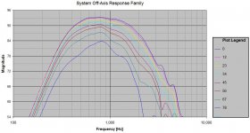
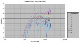
I recently began measuring my speaker projects on many axes in the horizontal and vertical planes. This helps me get a better idea of problem areas (holes or peaks) in the off-axis response. This information needs to be made available while you design the crossover (I think that is what you are showing above, not sure).
To address this need, I added some new functionality into my Active Crossover Designer tools to make it possible to import a number of off-axis measurements and see how the crossover influences all of the responses (both on and off-axis). Note that the data comes from actual measurements and not a model of the off-axis response for each driver.
I have attached two examples of this for a single driver with some EQ and filters added (e.g. not the system response). Please note that the version of ACD that can create these plots has not yet been released. There is also a new interface to generate surface and wireframe 3D plots instead of the line plots. I am waiting to get more experience with these new features, but everything is working well in my trials.
-Charlie
Attachments
Glad to see that people are finally starting to realize that an axial response alone is not enough to do a good crossover. Too much goes on off-axis that is important. I have been doing this for almost a decade now.
I use a finer set of data near the axis than further away since this is where one wants the better accuracy. I use 5 degrees up to 20, 10 degrees up to 60 and 20 degrees to 120, then 150 and 180. The data is then fit to a radiation model which yields 2 degree accuracy over the entire field. I only do horizontal polars currently as this is what matters most. There is always a pair of nulls above and below the horizontal plane and you have to look at these on occasion, but then one finds that they stay pretty well constant with the crossover point and separation distance and can be ignored for any other issues.
I use a finer set of data near the axis than further away since this is where one wants the better accuracy. I use 5 degrees up to 20, 10 degrees up to 60 and 20 degrees to 120, then 150 and 180. The data is then fit to a radiation model which yields 2 degree accuracy over the entire field. I only do horizontal polars currently as this is what matters most. There is always a pair of nulls above and below the horizontal plane and you have to look at these on occasion, but then one finds that they stay pretty well constant with the crossover point and separation distance and can be ignored for any other issues.
Is there a link to download and play with it?
Unfortunately no, but maybe in the future.
I think that is what you are showing above, not sure.
Idea is to monitor simulated power response while playing with cross-over components and topology.
Glad to see that people are finally starting to realize that an axial response alone is not enough to do a good crossover. Too much goes on off-axis that is important. I have been doing this for almost a decade now.
I use a finer set of data near the axis than further away since this is where one wants the better accuracy. I use 5 degrees up to 20, 10 degrees up to 60 and 20 degrees to 120, then 150 and 180. The data is then fit to a radiation model which yields 2 degree accuracy over the entire field. I only do horizontal polars currently as this is what matters most. There is always a pair of nulls above and below the horizontal plane and you have to look at these on occasion, but then one finds that they stay pretty well constant with the crossover point and separation distance and can be ignored for any other issues.
Hi Earl,
Say, you mentioned that you fit your measurements to a radiation model. Was this to calculate the power response? Now that I am paying more attention to off-axis responses, I am wondering what the best way to calculate the power response is. Just that just take lots of measuring and a manual integration of the results or is there a better way.
If that is not what you use the radiation model for, then when is that for?
-Charlie
Hi Charlie, that is a really good question.
When I started looking at polar responses and polar maps, I realized that I needed a higher resolution. One can always do 2 degree increments of measurements, but there had to be a better way.
Think of it this way; at LFs every two degrees is a total waste because the polar response just cannot change that fast with angle. But at HFs every two degrees is just about right because things can change this fast in the far field.
Interpolation comes to mind, but this is dangerous since diffraction effects have nulls that change in angle with frequency. So you can't just simply interpolate across the angles from FFT data as this will give you erroneous results. What I came to realize was that by expanding the polar radiation into what are called radiation modes - which are orthogonal and known everywhere - one can get a very good model of the radiation field and interpolation is not required.
Think of it this way, there is the monopole mode which dominates at LFs since the other modes are extremely inefficient, but then as the source get more directional a dipole mode comes into play. Then a quadra-pole mode, etc. I found that I could model the source very accurately up to > 10 kHz with about 16 modes (this is evident because adding more modes does not change the pattern. To calculate 16 modes only requires 16 points.
But in looking at the "modes" being fit (in "modal" space), the higher order ones are dominated by the forward direction. So I use a finer data spacing in the forward direction than in the rearward direction. I use 0, 5, 10, 15, 20, 30, 40, 50, 60, 80, 100, 120, 150, 180. This is only 14 points, but it still works well.
With the fitted polar model I can get a polar map resolution to about 2 degrees of resolution from 0 - 180 degrees with only 14 measurements instead of 90.
But wait, there is more!
It turns out that the sum of the squares of the modal coefficients is exactly the power (see Morse "Vibration and Sound" Eq 27.18). So I get the power response for free!
There's more.
Since I have the radiation modes, and they are valid everywhere, I can calculate back to the approximate source and see how the source was vibrating to create the sound field at any given frequency. This has been a tremendous advantage in tracing down aberrations and their cause. For example, in one speaker I had a small lull in the polar response at about 350 Hz and I was not sure what was causing this. By looking at the modal data I could see that it was caused by a quadrapole mode adding out of phase to the monopole mode. I could see that the cabinet was actually pumping front to back and side to side, a sort of breathing mode. A little stiffening and this went away.
So what I started out doing was one thing and what I ended up with was a very pleasant surprise.
The current model is only axisymmetric because in my speakers this covers about 90% of the polar map situation. But I plan on going to a full 3-D capability because only a few non-axisymmetric modes would be required right around the crossover to model the vertical nulls. Basically this should only take another 4 measurements, two up and two down, and I can nail the full 3-D polar response and power response.
Non-symmetric systems add a whole lot more complexity, but fortunately I don't ever deal with those.
Did you guys notice that kimmosto uses 360¤ measurements with even intervals. Earl says he uses bigger intervals far off and back horizontally. And how about verticals?
What is the "right way" to sum up power response? Is there a general agreement of that? What about "weighted" measurements?
Power response can be equal but radiation pattern may be different - will these speakers sound different in a room with reflections?
What is the "right way" to sum up power response? Is there a general agreement of that? What about "weighted" measurements?
Power response can be equal but radiation pattern may be different - will these speakers sound different in a room with reflections?
Power response can be equal but radiation pattern may be different - will these speakers sound different in a room with reflections?
That's the million dollar question. In my experience, yes, they sound different. I don't have a good answer how to correlate perception to such data but I'm sure others do
")
What is the "right way" to sum up power response?
"Right way" is to measure 4pi (hor & ver) power average with equal and narrow angle intervals. BUT if you are aware that the speaker is e.g. cardioid or front wall of your listening room is heavily damped and you don't care about actual SPL of power response, you are free weight front sector. Verticals should be included in simulation and final power response meas in order to make an excellent speaker without subjective X/O tuning.
I've also made simple investigation, how many measurements is enough to get acceptable power response estimation. Background for this was limit of 20 measurements per driver in LspCAD 6. Conclusion with regular 3-way was that 37 (0-180 step 10) horizontal measurements per driver is okay for X/O simulation. LspCAD is able use max 20, which could be without front/back weighting:
hor 0, 20, 40, 60, 80, 100, 120, 140, 160, 180 deg
ver +30, -30, +60, -60, +90, -90, +120, -120, +150, -150 deg
Vertical angles are constructed in LspCAD using horizontal measurements and drivers vertical location (time difference & directivity), to enable playing with locations/lobing.
Last edited:
37 (0-180 step 10)
Oops, 0-180 step 10 is only 19 measurements. I was thinking 5 deg steps which I use for directivity waterfalls.
- Status
- This old topic is closed. If you want to reopen this topic, contact a moderator using the "Report Post" button.
- Home
- Loudspeakers
- Multi-Way
- Nearfield/Farfield curve splicing