BJT SPICE Models, reality-check

[klewis]

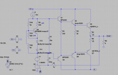
That was interesting. In the VAS, you are applying positive feedback instead of negative feedback (your image is wrong it seems). Try this.

I used different models, so you'll have to change them back.

- keantoken

Keantoken,

Thanks for the help. I got it to run in what I would describe as a static state - no input signal. So, how do I inject the sine wave into the model to get THD?

Ken

 

[keantoken]

Pretend the - side of the voltage amplifier is the input side of an LTP, so attach the input cource to it. Treat this voltage source as a VAS also, thus Cdom as C1. This gives proper compensation, whereas the old 1u cap actually did the opposite of compensation. I'm not sure how this schematic came about but it has some major errors.

- keantoken

 

[klewis]

Pretend the - side of the voltage amplifier is the input side of an LTP, so attach the input cource to it. Treat this voltage source as a VAS also, thus Cdom as C1. This gives proper compensation, whereas the old 1u cap actually did the opposite of compensation. I'm not sure how this schematic came about but it has some major errors.

- keantoken

It came from here
http://www.diyaudio.com/forums/solid-state/71534-semi-thermaltrak-52.html

post 519.

Thanks again for the help.

Ken

 

[klewis]

Keantoken,

It works great, thanks. Back to topic, do you have better models for the MJL3281/1302, MJE15033/32?

Ken

 

[keantoken]

These are models made by AndyC. The 4793/1837 are the drivers I usually simulate with, models also courtesy of Andy. These are all I have.

.MODEL mjl3281a_x npn IS=9.8145e-12 BF=438.0 NF=1.00 VAF=38 IKF=19.0 ISE=1.0e-12 NE=1.1237388682 BR=4.98985 NR=1.09511 VAR=4.32026 IKR=4.37516 ISC=3.25e-13 NC=3.96875 RB=3.997 RE=0.00 RC=0.06 XTB=0.115253 XTI=1.03146 EG=1.11986 CJE=1.144e-08 VJE=0.468574 MJE=0.34957 TF=2.6769e-9 XTF=7500 VTF=3.0 ITF=1000 CJC=1.093685e-9 VJC=0.623643 MJC=0.482111 XCJC=0.959922 FC=0.1 CJS=0 VJS=0.75 MJS=0.5 TR=1e-07 PTF=0 KF=0 AF=1 Vceo=200 Icrating=15 mfg=OnSemiconductor
.MODEL mjl1302a_x pnp IS=9.8145e-12 BF=122.925 NF=1.00 VAF=40 IKF=19 ISE=9.18577762370362E-07 NE=5.0 BR=4.98985 NR=1.09511 VAR=4.32026 IKR=4.37516 ISC=3.25e-13 NC=3.96875 RB=3.30 RE=0.00 RC=0.06 XTB=0.115253 XTI=1.03146 EG=1.11986 CJE=1.561e-08 VJE=0.781803 MJE=0.433868 TF=3.257e-9 XTF=1000 VTF=2.0 ITF=260 CJC=2.346838e-9 VJC=0.27876 MJC=0.411324 XCJC=0.959922 FC=0.1 CJS=0 VJS=0.75 MJS=0.5 TR=1e-07 PTF=0 KF=0 AF=1 Vceo=200 Icrating=15 mfg=OnSemiconductor
.MODEL Q2SA1837_x PNP ( IS=2.39372559E-10 NF=1.304015937 BF=300 VAF=273 IKF=2.087725944 NK=0.94719458 ISE=1.46829699E-11 NE=1.526663542 BR=4 NR=1 VAR=20 IKR=1.05 RE=0 RB=1.8 RC=1.65 CJE=4.7407E-10 VJE=1.1 MJE=0.5 CJC=8.6700E-11 VJC=0.3 MJC=0.3 TF=1.642191E-09 FC=0.5 ITF=1.076260106 XTF=5.868994022 TR=1.38U)
.MODEL Q2SC4793_x NPN ( IS=1.8E-09 NF=1.43 BF=146.38 VAF=273 IKF=2.6 NK=0.95 ISE=6.286997E-10 NE=2.223629 BR=4 NR=1 VAR=20 IKR=1.05 RE=0 RB=1.7 RC=1.25 CJE=5.96964E-10 VJE=1.1 MJE=0.5 CJC=5.78E-11 VJC=0.3 MJC=0.3 TF=1.22678E-09 FC=0.5 ITF=10 XTF=99.52253015 TR=983N)

- keantoken

 

[tiefbassuebertr]

an interesting thread
in this case this thread could be of interest:
http://www.diyaudio.com/forums/soli...ling-how-do-i-generate-p-spice-parameter.html

 

[klewis]

keantoken,

Happy new year a day early...

I'm trying to make my own models. Following Andy_C's instructions, I was able to plot hFE vs Ic, but can't figure out what expressions to use for the following:

1. Plotting Vbe vs Ic

2. Plotting B (Beta) vs Ic

3. Plotting fT at Ic = 100mA and 300mA

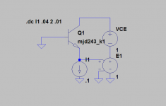
I'm sure you can help... the spice circuit setup is attached.

Thanks,

Ken L

 

[keantoken]

For Vbe vs. Ic, just click at the Q's emitter. Left-click on the bottom ruler in the trace window and deselect the logarithmic option (for other graphs the X axis is usually logarithmic, but not for Vbe).

Hfe and Beta are the same in andy's article if I'm correct, and it worked for me usually.

Now for Ft, set up a .ac analysis, right-click on I1 to give it the desired current, and then plot Hfe (Ic/Ib). Ft will be, if I'm correct, the point where Hfe crosses zero.

I can give a file to test Vcesat as well.

What is your aim though with the MJD models? I think I checked and they are surprisingly accurate compared to the throw-away models one usually encounters. (not to say there's nothing more to be desired...) And BTW you may be interested in the BD787/788 which are very similar, in fact they could be the same die, I had a hard time trying to find the difference.

This can get tricky since Andy doesn't describe the relationships simply between IKF, ISE, NE... Just so you know, I have some experience here and can help if necessary. (there are a few things I can't figure out myself though, which makes me wonder how on earth I managed to finish my 5769/5771 models...)

And by the way, I generally use the _k signature on my models to distinguish between them and the old models. It might be confusing if we use the same signature, if it matters.

And I ask you put finished model here, so other people can access them:

Spice Models - diyAudio Contributions - diyAudio

- keantoken

 

[klewis]

For Vbe vs. Ic, just click at the Q's emitter. Left-click on the bottom ruler in the trace window and deselect the logarithmic option (for other graphs the X axis is usually logarithmic, but not for Vbe).

Hfe and Beta are the same in andy's article if I'm correct, and it worked for me usually.

Now for Ft, set up a .ac analysis, right-click on I1 to give it the desired current, and then plot Hfe (Ic/Ib). Ft will be, if I'm correct, the point where Hfe crosses zero.

I can give a file to test Vcesat as well.

What is your aim though with the MJD models? I think I checked and they are surprisingly accurate compared to the throw-away models one usually encounters. (not to say there's nothing more to be desired...) And BTW you may be interested in the BD787/788 which are very similar, in fact they could be the same die, I had a hard time trying to find the difference.

This can get tricky since Andy doesn't describe the relationships simply between IKF, ISE, NE... Just so you know, I have some experience here and can help if necessary. (there are a few things I can't figure out myself though, which makes me wonder how on earth I managed to finish my 5769/5771 models...)

And by the way, I generally use the _k signature on my models to distinguish between them and the old models. It might be confusing if we use the same signature, if it matters.

And I ask you put finished model here, so other people can access them:

Spice Models - diyAudio Contributions - diyAudio

- keantoken

I think my model is way, way off, but, I'll get there... I couldn't figure out your instructions... could you make plt files, save them and send them back?

I've attached the sim files with the one plt file I have - the hFE vs Collector current.

If I every have a model worth sharing, I'll append it with either KL or K3

Thanks

Ken L

 

[klewis]

And now the file

 

[keantoken]

First, generally the Y-axis is usually not logarithmic, so they might look weird. (to change the law of you axis, you click the rulers at the edge of the trace window, and it brings up a box. And notice I said left-click, not right-click)

I don't know why you're messing with .plt files, I never even knew they existed! All you do is enter the equation Ic(Q1)/Ib(Q1), and you've got Hfe vs. Ic. The X-axis will always be the value of I1, because you're running a sweep simulation and that's the source that's being sweeped.

What exactly did you misunderstand?

- keantoken

 

[andy_c]

Now for Ft, set up a .ac analysis, right-click on I1 to give it the desired current, and then plot Hfe (Ic/Ib). Ft will be, if I'm correct, the point where Hfe crosses zero.

Tip for LTspice: To compute fT, simply set up a DC bias circuit for the device under test, making sure that Ic and Vce are set to the desired values. Perform an operating point simulation (.op). Then do a View, SPICE error log. The error log will show the fT of the transistor at the given operating point. Note that there's no way to plot fT vs. Ic in LTspice, so it's necessary to do it for one Ic value at a time.

This can get tricky since Andy doesn't describe the relationships simply between IKF, ISE, NE... Just so you know, I have some experience here and can help if necessary.

As I see it, the main difficulty with matching simulated and measured beta is that the equations for the Gummel-Poon model express Ic as a function of Vbe and Ib as a function of Vbe. So one must do the following:

1.) Pick a Vbe value.
2.) Compute Ic from Vbe.
3.) Compute Ib from Vbe.
4.) Compute beta = Ic/Ib.

Because one starts with Vbe, one does not know Ic exactly until it's computed in step (2) above. Since the formulas for Ic and Ib are explicitly known as a function of Vbe, we can take the ratio of Ic/Ib and say it is also explicitly known as a function of Vbe. But the structure of the formulas means that beta is an implicit function of Ic.

One way of getting around the problem of beta vs. Ic being an implicit function was created by Teodoro Marinucci (teodorom). It is as follows:

1.) Pick an Ic value.
2.) Solve for Vbe in the collector current equation using numerical root finding.
3.) Plug this Vbe value into the expression for Ib as a function of Vbe to determine Ib.
4.) Take the ratio Ic/Ib to determine beta.

The above technique doesn't work well with Excel and requires math software such as Mathcad, Mathematica or Matlab.

 

[klewis]

I got stuck at Andy_C's Ic vs Vbe and B vs Ic;

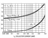
step 7. Using the circuit of Figure 11, plot Vbe vs Ic. How do I do this? I'm presuming that I want the y axis to be volts and the x axis to be Amps.

I understand how to change scales, I don't know how to describe a math expression of "vs."

Sorry for being so thick.

Ken L

 

[andy_c]

I understand how to change scales, I don't know how to describe a math expression of "vs."

If you want to change the quantity on the x-axis of an LTspice plot from its default, it becomes a so-called "parametric plot". I'm going to be a bit lazy responding here. In the LTspice help, choose the "search" tab. Enter the word "parametric" (without quotes) in the "keyword to find" box. You should see one topic, "Axis Control" come up. Check out the instructions for parametric plots found there.

 

[keantoken]

Vs. simply means a graph of Y vs. X.

So Ic would be the X axis and Vbe would be the Y axis.

- keantoken

 

[klewis]

So, I figured it out, I was trying to plot Ic instead of Vbe, plotted Vbe and put Ic on the bottom plot. The voltage reads negative, so I multiply it by -1 to get positive and it looks like the plot in data sheet. Do I have this right? I'm measuring the voltage at the emitter of the transistor for Vbe, and Ic is the current at the collector of the transistor.

If I have the above correct, then, I running into another issue, the maximum current in the model is somewhere around 3.4A, where the data sheet shows it going out to at least 4A and probably beyond. I haven't found the variable that will move this out further. Any thoughts?

 

[keantoken]

Two variables come to mind, Rb and Ikf.

I suggest you remove Ikf, Ise, and NE from the model temporarily... And follow the instructions copied from Andy's page:

Improved SPICE Models for MJL3281A and MJL1302A - Section 3

1. Keep the manufacturer’s model values for the device’s forward parameter VAF and reverse parameters BR, NR, VAR, IKR, ISC and NC.
2. Assume NF = 1
3. Permanently remove RBM and IRB from the model.
4. Set RB initially to zero and temporarily remove IKF, NE, and ISE.
5. Pick an initial value for BF equal to the maximum measured β at room temperature.
6. Start with the manufacturer’s value of IS.
7. Using the circuit of Figure 11, plot VBE vs. IC.
8. Adjust IS so that VBE at IC = 100 mA matches the datasheet value.
9. Adjust RB so that VBE at IC = 1 A matches the datasheet value.
10. Using the circuit of Figure 11, plot β vs. IC.
11. Adjust IKF so the reduction of β at high currents matches the datasheet as closely as possible.
12. Using the circuit of Figure 11, plot VBE vs. IC.
13. Adjust IKF and RB so that the VBE values at IC = 1A and IC = 10 A match the datasheet values as closely as possible.
14. Change the setup of Figure 11 so that the VCE source takes on values of 5 V and 20 V.
15. Adjust VAF so that the variation in VBE at IC = 20 A as VCE goes from 5 V to 20 V matches the datasheet.
16. Change the setup of Figure 11 back so that VCE is fixed at 5 V again.
17. Plot β vs. IC.
18. Adjust ISE, NE, IKF and BF so that β vs. IC matches the datasheet as closely as possible.
19. Plot VBE vs. IC.
20. Adjust IS, IKF and RB so that the VBE values at IC = 100 mA, IC = 1A and IC = 10 A match the datasheet value as closely as possible.
21. Repeat steps 17 – 20 until both VBE vs. IC and β vs. IC match the datasheet as closely as possible.

If you leave IKF, ISE and NE in you will be dealing with with a multidimensional nightmare... So start with Is to get the Vbe right, and go from there.

We generally start with an otherwise perfect model, tweak the Vbe variables to make it perform like the device at low currents, and then add the high-current behavior parameters.

- keantoken

 

[keantoken]

I also suggest you put this command in:

.temp -40 25 125

This will let you adjust the tempco parameters to fit the datasheet when and if possible.

So first on the list is:

1: Adjust Is to match the datasheet at negligible currents.
2: If necessary and if possible, adjust Eg to match all three temperature plots. (Eg is generally constant between BJT's, but there are a few exceptions)

- keantoken

 

[klewis]

keantoken and Andy (if you're following)

question for you:

for the MJL3281, does HFE rise with voltage? I tried Andy's model at 50v it showed hFe of 228 at 10A. The spec sheets aren't much help...

see my post here:

http://www.diyaudio.com/forums/chip-amps/143947-lme49810-std03-parallel-pairs-7.html#post2042177

Ken

http://www.diyaudio.com/forums/chip-amps/143947-lme49810-std03-parallel-pairs-7.html#post2042177

 

[keantoken]

IIRC, Hfe linearity improves with higher Vce, and there is also Early affect. This parameter would be Vaf in the model.

- keantoken