Tweaked KSC1845 / KSA992 LTSpice models

[cabirio]

Hi all,

I've recently bought a Peak atlas DCA Pro transistor tester and after playing with it for a while, I thought I'd have a go at tweaking some LTSpice models based on actual measurements. I've started with the KSC1845 / KSA992, since I have a bunch and they seem to be popular around these parts.

What I've done is based mostly on Bob Cordell's superb book "Designing Audio Power Amplifiers" and various DIYA contributions from Keantoken, Andy_C, Dave Zan and many others to whom I'm forever grateful for sharing their knowledge. Please note that this is my first attempt and I'm far from an expert, so the usual disclaimers apply: as far as I can tell, the models are much closer to reality than the stock ones (*), and so far they've worked fine in all the various simulations I've used them in, but I'll take no responsibility if using them sets your house on fire or something. Comments and corrections are of course welcome.

I don't want to make this first post too long so I'll give more details later (of course Bob's stuff is published material so I'll just go into things he doesn't cover or I've done differently), just a few initial comments to get things started:

- At the moment I have 10 x KSC1845 and 15 x KSA992. First I took a quick hFE / Vbe measurement of all of them and picked the ones closest to the average to measure in more detail and base the models on. They are both gain group F and have an hFE of around 400.

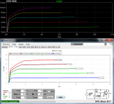
- As you can see, both have quasi saturation. It is well known that LTSpice's qs modelling has its problems, some of which I'll go into in more detail later. fT modelling in particular is directly affected by qs, and in the case of the KSC1845, so much so that it's impossible to get an fT curve that peaks where it should. For that reason I've also created a model without qs, which could be useful in cases where bandwidth, phase margin, etc. are more important than qs.

- It's frustrating that datasheets rarely (if ever) give any useful info about reverse characteristics, but I always assumed those parameters wouldn't matter much in the usual circuits. Then one day I modified by accident ISC in one of my models and the forward curves, the qs region in particular, changed quite a bit. I came up with a little trick to make the DCA Pro plot reverse curves, so I've had a go at tweaking those parameters too.

- Where neither the datasheet nor my measurements gave me useful info to adjust some parameter, I either left it at its stock or default value, followed Bob's very useful rules of thumb or just made an educated (I hope) guess. I realize that some things require building a specific measurement rig (the DCA Pro has its limitations) but I wanted to see how far I could get with what I have.

So, without further ado:

.model KSC1845 NPN (
+IS = 52.5f NF = 1.0 BF = 408 VAF = 150
+ISE = 4f NE = 1.5 IKF = 0.8
+RC = 0.28 RE = 0.15 RB = 40 RBM = 4.0 IRB = 250u
+ISC = 1.9p NR = 1.0 BR = 15 VAR = 20 NC = 1.3
+CJC = 4.8p VJC = 0.6 MJC = 0.29 TF = 149p VTF = 4.0
+CJE = 26.5p VJE = 0.73 MJE = 0.162
+RCO = 105 VO = 2.2 GAMMA = 1.6u QCO = 2p QUASIMOD = 1
+EG = 1.181 TR = 10n XTB = 1.728 )

.model KSC1845NQ ako:KSC1845 (
+RCO = 0.0 IKF = 0.39
+CJE = 31p TF = 418p ITF = 68m XTF = 18.7 )

.model KSA992 PNP (
+IS = 48.3f NF = 1.0 BF = 395 VAF = 65
+ISE = 0.5f NE = 1.5 IKF = 0.25
+RC = 48m RE = 4.4m RB = 25 RBM = 2.5 IRB = 3.8m
+ISC = 1.8p NR = 1.0 BR = 5.9 VAR = 12 NC = 1.3
+CJC = 7p VJC = 0.6 MJC = 0.32 TF = 365p VTF = 4.0
+CJE = 25p VJE = 0.855 MJE = 0.4404 ITF = 0.75 XTF = 1.13k
+RCO = 55 VO = 3.0 GAMMA = 490n QCO = 300f QUASIMOD = 1
+EG = 1.16 TR = 10n XTB = 1.285 )

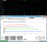
KSC1845NQ is the one without quasi saturation. See attached simulated (top) and measured (bottom) Ic vs Vce curves. More to come...

(*) https://www.onsemi.com/pub/Collateral/KSC1845.lib
https://www.onsemi.com/pub/Collateral/KSA992.lib

 

[cabirio]

Ok, one thing at a time. For the first three lines in the models (I've arranged the parameters in what I think is a logical way) I pretty much followed Bob's steps. One thing to note is that with the stock RB / RBM / IRB, I had some trouble to match the low and high base current Vbe measurements. In this thread Richard Marsh measured noise and extracted Rb for a bunch of transistors, and Keantoken kindly made a summary here. Since the KSC/KSA are often recommended as modern replacements for the 2SC2240/2SA970, also marketed back then as low noise and with not too far off characteristics, I just took those values, 39 (rounded to 40) and 25, respectively, for my RBs. For RBM I figured 1/10th of RB (I have found very little information on the decrease of Rb at high base currents, but Dave Zan has often commented on RBMs of just a few milli-ohms being unrealistic, so I thought 1/10th is still a significant resistance, probably?) and then adjusted IRB to get my high current Vbe right. A lot of guesswork here, so don't expect the models to give you accurate results in noise simulations.

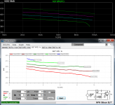
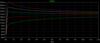
One of the measurements the DCA Pro provides is hFE vs Ic for different Vce values (attached). The first thing to note, and this has been commented on by e.g. Douglas Self in APAD, is that LTSpice models Early voltage as a linear effect, which it clearly isn't. However the plot is very useful to adjust VAF, which sets the spacing between the traces, as well as the low and high hFE droop parameters. As it is impossible to match each trace, I just went for something that matches visually the measurement as well as it can match it. There was some back and forth with the Ic vs Vce traces too.

I'm not sure why these traces are so jagged. I suspect that, because the collector bias is provided via a 700R resistor (see the little schematic at the bottom right), adjustments have to be made to the voltage source on the fly as Ib increases to keep Vce at the right value. I may drop a line to Peak to ask them about it.

The funny wiggle at the end of the bottom trace in the KSC is due to qs, which at this point I had already started adding to the models. More in the next episode...

 

[cabirio]

There is an often cited paper about modelling quasi saturation: G.M. Kull, L.W. Nagel et al., "A unified circuit model for bipolar transistors including quasi-saturation effects". I got it and had every intention of reading it, but searching DIYA I came across a very succint, visual explanation of what the qs parameters do, courtesy of Keantoken (many thanks again!), here. I was impatient to start playing with this so I never studied the paper in detail, maybe one day...

Anyway, I can't explain it better than those pictures. Unfortunately, because the parameters interact not only between them but also, as I said above, with the reverse parameters (ISC, NR, BR, VAR, NC), I can't give you any rules of thumb about starting or typical values. FWIW, I've played with it in maybe a couple dozen of models (which I'll refine and share when I think they're ready) and I have RCOs ranging from 3 to 350, GAMMAs from 5n to 550u and VOs from 0.7 to 40.

Now for the problems. One is what happens when you have your traces looking good for a given, reasonable Ic range and then see what happens at higher currents (attached picture #1 is the KSC1845 with Ib = 50 mA to 250 mA). Hmm... Things seem to improve if you increase VO, but this will require you to also increase GAMMA and RCO to match the original traces, and the match won't be as good, especially at lower currents, and although things do improve and the artifact is reduced, it doesn't disappear completely. So, as always it's a compromise: how important it is for the circuits you plan to use the model in what happens in some range of operation vs. another one. In this particular case, I don't see myself asking a small signal transistor to deliver more than a few mA, so I'm not too concerned about it.

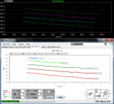
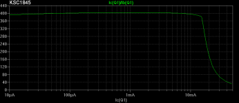
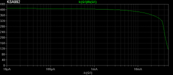
Another feature (rather than problem, I think) of qs is what it does to the hFE curve (attached pictures #2 and #3). If you look at the datasheets (*) you will see that the KSC1845 does have a sharp knee from around 8-9 mA, but my model has it higher, sharper and with a different shape. You can manipulate the qs parameters and get a better match, but then your Ic traces will be off. Again, it's a compromise. The case of the KSA992 looks better though, perhaps because the qs effect is not as pronounced or because of the particular combination of parameters, I haven't really looked into this in much detail.

Finally there's the glitch in the fT curve, but I'll look into it in another post (this is where the QCO parameter comes into play). As for QUASIMOD, it's just a flag to enable the temperature dependence of qs, which the paper above claims is well characterized, so it seems like a good idea to include it.

Next up: reverse operation...

(*) https://www.onsemi.com/pub/Collateral/KSC1845-D.pdf
https://www.onsemi.com/pub/Collateral/KSA992-D.pdf

 

[cabirio]

A nice feature of the DCA Pro is that you connect the leads to the transistor however you want and it automatically identifies the C, B and E terminals. The trick to make it give you reverse traces is simply to swap the C and E after the initial test, apparently it doesn't re-check before each measurement.

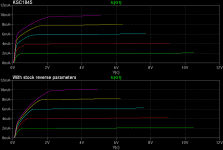
The Veb breakdown voltage of these transistors is 5V, but to keep things safe I run the tests up to 2V only. ISC and NC work pretty much like ISE and NE, setting the low current beta droop amount and shape. NR, BR and VAR correspond to NF, BF and VAF. Note that, as has been commented elsewhere (I can't find it now, I believe this was an exchange between Keantoken and Dave Zan) for the model to work properly NR has to have the same value as NF. What happens if they aren't is that the whole set of forward and reverse traces are shifted with respect to the (0, 0) origin and they don't cross it, which doesn't make physical sense. So, if you tweaked NF, don't forget to set NR to the same value. IKR corresponds to IKF and sets the reverse high current beta droop. As I can't run traces at high reverse current due to the 700R resistor, I can't adjust it, so I simply removed it, which makes it default to infinity. It doesn't seem to affect anything in the forward traces until it's small enough to affect the reverse ones.

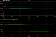
To illustrate the influence of these on the forward curves that I mentioned above, see what happens when I change all reverse parameters to their stock values (attached pictures #3 and #4). The effect on qs is obvious and note that, even without qs, there is an impact both in overall gain and in the shape of the traces as they approach 0.

 

[cabirio]

And finally the frequency related stuff. I'll start with CJC / VJC / MJC, since these aren't affected by any other parameter (for a change!) but they do affect the fT curve, so they should be dealt with first.

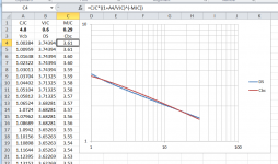
Here I do things differently from Bob Cordell, to get Cbc to fit over a larger range. Basically I use FPGraphTracer to capture the Cob vs Vcb curve, then feed the values into a little spreadsheet I made (attached picture #1) with the formula used by LTSpice, Cbc = CJC * (1 + Vcb/VJC)^(-MJC), and tweak the parameters for the best fit. CJC shifts the whole curve up and down, VJC affects the flatness and MJC controls the slope. Don't expect a perfect fit but I'm pretty sure something like what's shown in the picture is more than close enough.

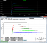
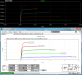
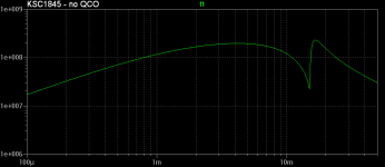
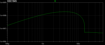
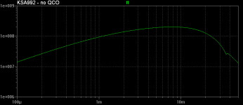
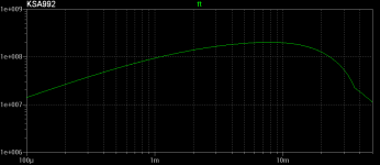
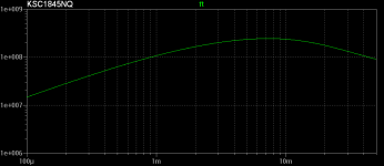
Then it's back to Cordell for TF, VTF, CJE, VJE, MJE, ITF, XTF. Once again Keantoken was kind enough to provide a very nice sim file that generates the fT curve here, which really helps a lot, and here's where things get interesting when you have quasi saturation. Attached picture #2 corresponds to the KSC1845 model without specifying QCO (it defaults to 0). Although the fit below 3 mA or so is good, that huge glitch looks like the kind of thing that could cause problems. Not that I've had any in the test circuits I've run, but I've never pushed the current that high, so, since QCO removes the glitch by flattening the curve after the notch (attached picture #3), I though it would be a good idea to include it. I just increased it until the jump was removed. Note that qs causes enough of a drop in fT that I removed ITF and XTF and even so I had to reduce TF quite a lot to get a good match at low currents. For the case of the KSA992 (attached pictures #4 and #5) as you can see the effect isn't as dramatic and here I was able to at least make the curve peak at the right current with the right fT value. For the KSC1845NQ model (attached picture #6) I just put back and adjusted ITF and XTF.

 

[keantoken]

I'm surprised I didn't see this.

It looks like you are on the right track. Itf and Xtf are the "old way" of modeling Ft when there was no quasi-saturation model. If your Ft droop occurs in the quasi-saturation region then the correct way to model it is with the quasi-saturation parameters. On the Sanken power transistor models I made, I even had to increase IKF to quite large values because I got the best fit when all the of the beta droop was explained by quasi-saturation.

Just a note, you probably need to add quasimod=1 to your models to make the quasi-saturation region react sensibly to temperature changes.

 

[cabirio]

I'm surprised I didn't see this.

It looks like you are on the right track. Itf and Xtf are the "old way" of modeling Ft when there was no quasi-saturation model. If your Ft droop occurs in the quasi-saturation region then the correct way to model it is with the quasi-saturation parameters. On the Sanken power transistor models I made, I even had to increase IKF to quite large values because I got the best fit when all the of the beta droop was explained by quasi-saturation.

Just a note, you probably need to add quasimod=1 to your models to make the quasi-saturation region react sensibly to temperature changes.

A rather belated thank you, keantoken. As suggested I did add quasimod=1 to these, as well as to all the models with quasi-saturation I just posted here.

Cheers,

Cabirio