I think they will both be varied by frequency.
Not for "digital delay", no.
"Digital delay" is just taking the audio samples and making them come out in order some time later. In the good old days this was called a "bucket brigade delay line". This does not alter the phase behavior at all except to add pure delay, which is independent of frequency.
You can use DSP to apply an all pass filter, or use FIR DSP to implement arbitrary phase responses with flat amplitude, but I do not believe that is what steveu was referring to.
By inspection of the transfer function equation you can see that there will be zeros at s = + and - infinity, and this is what pulls the response down for large positive and negative frequencies.
Maybe you can, but I can't. I only see poles. There is no value of s that makes the numerator zero.
Maybe you can, but I can't. I only see poles. There is no value of s that makes the numerator zero.
It's the value of the transfer function that should be zero at a zero, not necessarily the numerator (only).
If you plug in s=infinity, the expression evaluates to zero. So s=infinity is a zero of the function.
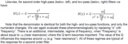
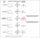
Attached is an excerpt from the technical manual for my crossover design tools, ACD, about second order filter transfer functions. Thinking of s like frequency, you can easily see how the functions give rise to highpass or lowpass forms, and where the function will have zeros. Only the highpass filter has a zero formed by the s^2 term in the numerator.
Attachments
How to find transfer function to use in the calculation? Is it derived from the circuit analysis, Kirchoff (KVL, KCL)? And then take it into Laplace transform to make it stay in s-domain, later substitute s with jw, is this the correct procedure to use pole-zeros analysis in crossover network?
It's the value of the transfer function that should be zero at a zero, not necessarily the numerator (only).
If you plug in s=infinity, the expression evaluates to zero. So s=infinity is a zero of the function.
But now you treat infinity as a number. s is normally taken to be a complex number, the real and imaginary parts of a complex number are by definition real and infinity is not an element of the set of real numbers as far as I know. Hence, no complex value of s will make the transfer function zero.
Of course I'm nitpicking, but that's just the point: I think everyone understands that the function tends to zero when s approaches infinity, but whether you regard that as the result of the factors in the denominator and hence of the poles, or come up with a description involving zeros at infinity is really a matter of taste.
How to find transfer function to use in the calculation? Is it derived from the circuit analysis, Kirchoff (KVL, KCL)? And then take it into Laplace transform to make it stay in s-domain, later substitute s with jw, is this the correct procedure to use pole-zeros analysis in crossover network?
Yes. Take the impedance of an ideal inductor to be sL, the impedance of an ideal capacitor to be 1/sC, apply Kirchhoff's laws and solve the set of equations. For most standard filters that has already been done and you can just look up the results in filter handbooks.
Maybe you can, but I can't. I only see poles. There is no value of s that makes the numerator zero.
There is a complex infinity and it can be used as 1/infinity =0
Riemann sphere - Wikipedia
Fair enough, but does it make any difference for a loudspeaker crossover filter whether you define its transfer function for complex values or for extended complex values of s? I don't think so, so both ways of looking at it, with or without zeros at infinity, are equally correct.
@ MarcelvdG: I can't quite understand why you find it an uncomfortable concept. I think it makes a lot of sense in a phenomenological way, as I will explain.
Think of a high pass filter. Any order you choose, but for my argument I will say first order. We all know that below the knee the response asymptotes to 20dB/decade or 6dB/octave. What happens if you keep going, and going, and going down the log frequency scale? Does this slope ever change (talking ideal not real world filter here, no losses, etc.)? The answer is no.
The only way to explain that is to have a zero located at zero frequency, which on the log f scale is infinitely "down there" in frequency. There is no "end" to the attenuation for our ideal filter, only infinite log attenuation, or zero amplitude, at f=0.
In the same way, consider a first order low pass filter. Above the knee the response has a slope of -20dB/decade, or -6dB/octave, and that is maintained "forever", that is to say out to "infinite" frequency where the log attenuation becomes infinite and the amplitude zero. This is because a zero is lurking there, like planet X. You can't see it (because it is infinitely far away) but you can see its effects on the response a bit closer in! 🙂
I can understand its usefulness for low-pass to high-pass transformations and vice versa, and it can also be useful when you start calculating integrals, but I think otherwise using extended complex numbers instead of normal complex numbers and having zeros at infinity just complicates matters.
For example, when you use normal complex numbers for s, it is immediately clear what is meant by an all-pole filter. With extended complex numbers, each n-th order filter has n zeros, so you get a tricky definition of all-pole filter: a filter that has all its zeros at infinity.
Without the zeros at infinity, the magnitude of H(s) is simply some constant factor times the product of the distances from the zeros to s divided by the product of the distances from the poles to s. With zeros at infinity, you have to treat infinite zeros different from finite ones.
Last edited:
And if you delay by a couple of hundred us, 10kHz will be down 180 degrees yet at 1kHz it will be almost unchanged. Like a physical displacement."Digital delay" is just taking the audio samples and making them come out in order some time later.
And if you delay by a couple of hundred us, 10kHz will be down 180 degrees yet at 1kHz it will be almost unchanged. Like a physical displacement.
We are talking apples and oranges now. Let's go back to your earlier post about this:
I think they will both be varied by frequency.
Which you wrote this in response to this part of my post:
Also, using pure delay does very little to nothing to "fix" or "cancel" phase distortion. That is because that kind of delay is independent of frequency, whereas the delay resulting from a crossover filter changes with frequency.
In the above posts, I am talking about delay: the "pure delay" of a digital delay, and the frequency dependent group delay of an electrical filter used in a crossover. I am not talking about phase, and I think this is where you are getting a bit mixed up.
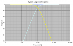
For example, let's look at the LR4 filter. Here are the magnitudes of the HP and LP filter functions:
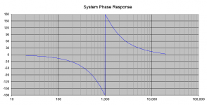
The filters sum flat. When you look at the phase response of the sum, it looks like this:
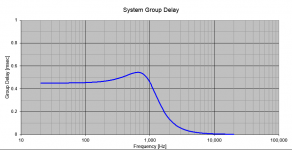
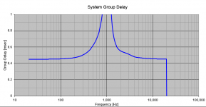
And from that you can generate the group delay, which looks like this:
As you can see, the group delay is not constant vs. frequency when you sum the HP and LP filters of the LR4 type. In fact, the following kind of general shape to the group delay response is generated by the sum of pretty much every HP+LP filter pair used in crossover networks:
- At frequencies far below the crossover point the group delay is more than at frequencies far above the crossover point.
- There is a transition region around the crossover point. There may be a peak in the group delay in this region, especially if the filter has higher Q stages (Q>1).
- The group delay falls back to almost zero at the highest frequencies.
What I mention in the last quoted post of mine, above, was the fact that it is not a good correction to use digital delay (flat line) to correct for the group delay curve of a filter sum (not flat line). You might think that you could just delay the tweeter (F>Fc) and that would increase its delay to match the woofer (F<Fc) but what happens is that, while you can get the GD at high frequencies to equal the GD at low frequencies you exacerbate the peak at the crossover frequency quite a lot. This is just making a bad situation worse. For example, I did this and here is what you get 😱
To equalize (flatten) the group delay filters you need some additional network having a group delay profile that starts out at zero at low frequencies and then ramps up at just above the crossover point to a level about what the GD is for the woofer (the LP filter part of the summed filter response). A sort of "inverse" to the LR4 group delay I plotted above. But there is no practical "analog" filter that can generate that group delay profile shape and you must employ FIR filters to get it. But you could also have used FIR LP and HP filters from the start and designed them to have flat group delay (aka linear phase).
Phase distortion was mentioned above. This is just the consequence of frequency dependent delay: some frequency components in the waveform will emerge at a different time (e.g. later) than other frequency components.
Attachments
But there is no practical "analog" filter that can generate that group delay profile shape and you must employ FIR filters to get it.
That is not fully true as Meyer and PSI have shown. But I must admit that it is not easy.
Unfortunately there is no reliable information yet what group-delay shape is below audibility for everyone. Such an information would be of great help in designing crossovers that are audibly "blameless" (sorry Douglas S. for stealing the term) but probably simple in construction.
There was once a paper by the German institute for broadcast technology (IRT) asking for a deviation of less than +- 200us from linear between 700 Hz and 7kHz but that was based on theoretical studies and not on listening tests. But that is a value that is reachable by analog crossovers of certain topologies.
Regards
Charles
I think otherwise using extended complex numbers instead of normal complex numbers and having zeros at infinity just complicates matters.
Another complication is addition: for complex numbers, a + b = a + c is equivalent with b = c, for extended complex numbers that is not necessarily so, as infinity + 3 = infinity + 5.
Well, as an example, in thus forum within the past year I raised this same point and someone said "ah but I have a program to design all pass (analog style) filter banks that can satisfy any delay shape you want!". So I posted a simple one like the LR4 above and it took some huge order (like 20th order or 60th order or something) in order to get a good approximation. It's not really all that tractable a solution IMHO. That is why I didn't say it was "impossible" only that it was "impractical".That is not fully true as Meyer and PSI have shown. But I must admit that it is not easy.
I think that it's not the "shape" of the group delay profile that is of concern but rather the maximum group delay difference and even then I agree that there has been very little research into the audibility of that. From memory there was a study that concluded that the threshold of 1 or 2 msec around 1kHz became audible, but much more delay at lower frequencies e.g. below 100Hz was less audible and the threshold might rise up to 100 msec by 10Hz. Anyway, that topic could easily get its own thread. With FIR filtering it would be possible to cook up some ABX testing protocols using music.Unfortunately there is no reliable information yet what group-delay shape is below audibility for everyone. Such an information would be of great help in designing crossovers that are audibly "blameless" (sorry Douglas S. for stealing the term) but probably simple in construction.
There was once a paper by the German institute for broadcast technology (IRT) asking for a deviation of less than +- 200us from linear between 700 Hz and 7kHz but that was based on theoretical studies and not on listening tests. But that is a value that is reachable by analog crossovers of certain topologies.
Regards
Charles
When you say "that is a value that is reachable by analog crossovers of certain topolgies" I will just mention again that the designer should look at the entire loudspeaker system and try to optimize its group delay, if you are going to try to do that at all. There are contributions from the crossover filters as we have been discussing, but also from the driver offsets caused by the various setbacks of the acoustic centers, as well as the different pathlengths from those acoustic centers to the listener. The crossover does have a dominant role in the overall delay profile and it would be good for the designer to consider that source of group delay "misalignment" carefully. I concur that, without good data as a guide, it is difficult to know when delay variability is "good enough".
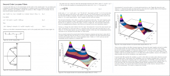
I found the attached paper one of the easiest to follow as far as understanding how filter transfer functions are plotted in the complex plain and relate to the frequency response. Also, there are two examples of going from passive first or second order filters to poles and zeros. An excerpt for 2nd order LP filter from the paper and a summary “cheat sheet” for other types of second order filters I found handy are also attached.How to find transfer function to use in the calculation? Is it derived from the circuit analysis, Kirchoff (KVL, KCL)? And then take it into Laplace transform to make it stay in s-domain, later substitute s with jw, is this the correct procedure to use pole-zeros analysis in crossover network?
Regarding the zero at infinity:
Back in college it was suggested to visualize the complex plane as a massless, elastic rubber sheet. For normalized filter transfer functions(ie gain = 1.0, or 0dB) the outer perimeter of the rubber sheet would be fixed to a hoop of “infinite radius” held at elevation of 1 above the floor plane. Zeros could be visualized as tacks fixing the rubber sheet to the floor at a point. Poles could be visualized as “infinitely” tall telescoping tent poles pushing up on the rubber sheet at a point. The magnitude of the frequency response is the height of the sheet above the floor as you move along the +jw axis starting from the origin (0,j0) .
So far so good…but what about the zero at infinity? Well, it isn’t a zero at a point(or 2 points), rather it is a zero around the entire perimeter of the complex plane. If the degree or order of the ‘s’ polynomial in the denominator is larger than in the numerator the hoop supporting the perimeter of the rubber sheet representing the complex plane would be moved from an elevation of 1, down to the floor(ie elevation = 0). LP and BP filters are examples of this. I’m not sure of the mathematical nuances that make this troubling, but if you make a carpet plot of a LP or BP transfer function, it is easy to see the value asymptotically approaching zero in all directions as you move away from the origin.
Of course the rubber sheet analogy breaks down as soon as you start dealing with filters containing more than one pole or zero at the same location. Despite that, it was a helpful mental visualization tool back in the day before you could easily create a carpet plot with a few keystrokes in Matlab or Excel.
Attachments
Any chance you can provide a link to this thread?...in thus forum within the past year I raised this same point and someone said "ah but I have a program to design all pass (analog style) filter banks that can satisfy any delay shape you want!". So I posted a simple one like the LR4 above and it took some huge order (like 20th order or 60th order or something) in order to get a good approximation.
Practical or not, I am interested to learn about the analog filter bank technique you mentioned, but have been unable to locate thru forum searches. Thanks!
Any chance you can provide a link to this thread?
Practical or not, I am interested to learn about the analog filter bank technique you mentioned, but have been unable to locate thru forum searches. Thanks!
It took me awhile but I managed to track it down for you. See post #8 in this thread:
How to correct phase for IIR filters
Another complication is addition: for complex numbers, a + b = a + c is equivalent with b = c, for extended complex numbers that is not necessarily so, as infinity + 3 = infinity + 5.
As it should be. And infinity times a divided by infinity times b is a divided by b.
This is used over and over in math, including transfer functions. Kinda like 1/x as x goes to zero, or infinity.
Last edited:
- Home
- Loudspeakers
- Multi-Way
- Pole-Zeros