I showed in #11 that the LP produces 3dB less signal at 800Hz as at 2Khz. So it’s not your Cart, it’s the LP.
Hans
Hans
@chip_mk,
The bulge in your FR around 20kHz can only be diminished by using a much larger capacitance.
Just start with an extra 330pF and see what it brings.
And instead of using the time consuming way to construct a FR in Audacity, you could load the recorded .wav file into RightMark Audio Analyzer which is freeware.
Load the .wav file with the most right option at the bottom called “Spectrum Analyzer” and it will process your 28 sec .wav file in one go.
Use the largest FFT size.
Hans
P.s. I forgot to say that within Audacity you will have to construct an upwards going 10dB/dec eq filter from 300Hz to 30Khz or so, to rotate the spectrum from 10dB/dec downwards going into a horizontal one. Once made, it will be a hit of a button in Aadacity to apply the filter.
Last edited:
Thanks for the advice. I hoped one day would find a proper setting and make Audacity -> Plot Spectrum work for the purpose. But will certainly try RightMark as recommended.
Regarding excessive HF peaking, it seems to me it's a mechanical resonance. I'm kind of skeptical taming it with electrical means. It would reduce the amplitude but the Q would remain the same. Impulse response would steel suffer.
And adding C would increase Q of the electrical resonance, possibly further deteriorating impulse response. For this reason, linearizing the FR curve is not guaranty for natural sound in my opinion. Reducing R could possibly diminish the peak without raising the electrical Q. Potentially lot of fun trying various combinations. Quite possibly, just accepting prominent HF end (as is) would appear to be most acceptable compromise sonically.
Don’t you worry about adding a larger capacitance, just try it, it won’t effect any mechanical resonance.
Maybe reading this article will give you some more background.
https://www.diyaudio.com/community/...vidual-transfer-functions.397815/post-7314673
Hans
Maybe reading this article will give you some more background.
https://www.diyaudio.com/community/...vidual-transfer-functions.397815/post-7314673
Hans
Sorry for my late response but what puzzles me in the spectrum analysis plot is the increase in noise starting around 10kHz and peaking around 20kHz.Sweep recorded with linear preamp (192kHz SR)
View attachment 1184934
Let's take a pinch of it, select ~100ms somewhere and use Analyze -> Plot Spectrum feature in audacity:
View attachment 1184935
Peak at 1001Hz suggests this is the part of the sweep around 1kHz. Now let's use Analyze -> Measure RMS option.
View attachment 1184936
Write down (insert in spreadsheet) that value. Then continue doing the same in other parts of the sweep. With 10-15 evenly spaced measurements one can make a decent plot. Here is one made with 56k || 22pF + 110pF(cable) input impedance with a linear preamp (Left blue, Right red)
View attachment 1184939
What surprises me the most is the deep below 2kHz. I don't know what causes it.
I have to clarify, the sound from LP I perceive as a kind of dull-ish when compared to CD. But it is evident only after comparison. Maybe this recessed mid is the cause of the subdued presentation.
What causes this?
Hi Joe,
That's because of the used logarithmic frequency scale.
When plotted an a linear scale, noise will be evenly distributed.
Hans
That's because of the used logarithmic frequency scale.
When plotted an a linear scale, noise will be evenly distributed.
Hans
Thanks for the advice. I hoped one day would find a proper setting and make Audacity -> Plot Spectrum work for the purpose. But will certainly try RightMark as recommended.
Regarding excessive HF peaking, it seems to me it's a mechanical resonance. I'm kind of skeptical taming it with electrical means. It would reduce the amplitude but the Q would remain the same. Impulse response would steel suffer.
And adding C would increase Q of the electrical resonance, possibly further deteriorating impulse response. For this reason, linearizing the FR curve is not guaranty for natural sound in my opinion. Reducing R could possibly diminish the peak without raising the electrical Q. Potentially lot of fun trying various combinations. Quite possibly, just accepting prominent HF end (as is) would appear to be most acceptable compromise sonically.
Years ago Scott Wurcer did a Python script to plot sweep FR - conceived around this post here. Recently we've extended it to support full-range sweeps, include (I)RIAA filters to accommodate various test records (though only at 96kHz for now), correction for the CBS-STR100 sweeps, and support to use a stereo file for each channel so that crosstalk can be plotted.
Requires Python but is simple to use once you understand how to set setup the files. You can find the latest code and Python installation instructions here.

That would be an interesting test record.
Mine would be +16 at 15khz or better if yours is plus 4. I tuned the RIAA curve to make LPs sound as live as CD. I used dire straights , Fleetwood mac and Steely Dan as test records.
Cart is Shure VM15 type 2.
Mine would be +16 at 15khz or better if yours is plus 4. I tuned the RIAA curve to make LPs sound as live as CD. I used dire straights , Fleetwood mac and Steely Dan as test records.
Cart is Shure VM15 type 2.
Indeed there's loads of goodies in scipy.signal for signal processing, both analog and discrete... Between numpy, scipy, soundfile and matplotlib you can do lots of interesting stuff. And numpy/scipy are heavily optimized C++ under the hood, used heavily in the scientific community so its rock solid.Requires Python but is simple to use once you understand how to set setup the files. You can find the latest code and Python installation instructions here.
This chart includes old and some new measurements for comparison. Input load is stated in the legend. Capacitance values are without cable capacitance which is additional 100pF. Lower resistance/higher capacitance load reduces the peak @20kHz and fills the 5-10kHz region and subjectively is more balanced (I have in mind 47k 220pF curve). Cartridge is Goldring G1012GX.

I recently bought the Ortofon test record. I was hoping to use REW to plot the response. I have yet to figure out how to do it but it looks like the import sweep function might work if I can generate a reference sweep of the same length and content as what is on the record. I may break down and find the python script mentioned in the earlier posts, but that is a royal PITA as those libraries are always changing and Python code rarely works for more than a year until some fool breaks the backward compatibility of the library.
ABSOLUTE PHASE:
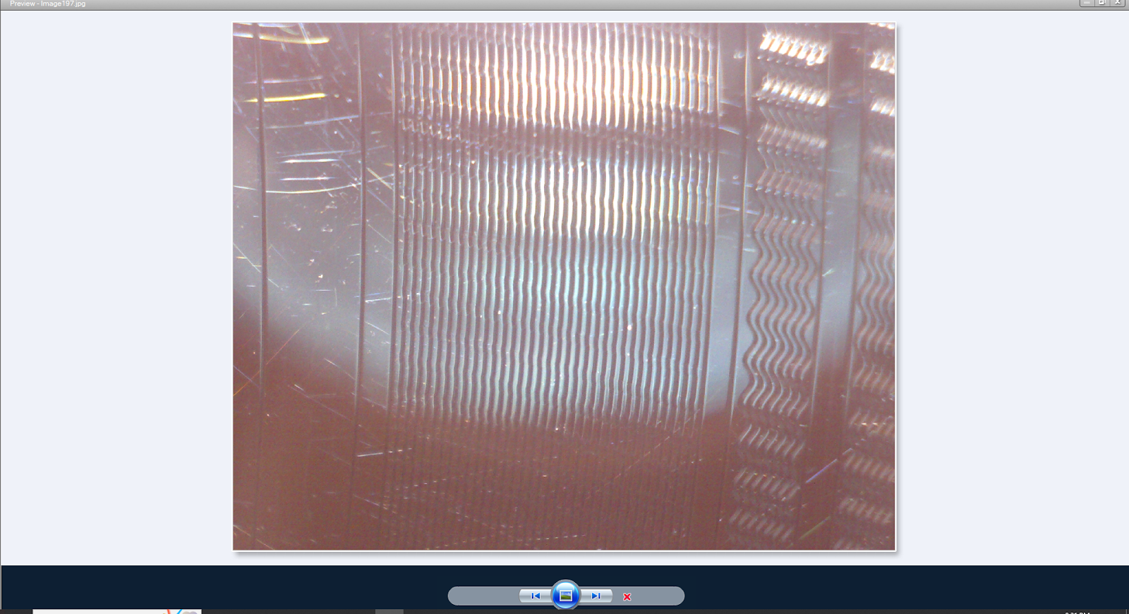
I wanted to use the last track to determine absolute phase for my system but the description of the waveform was useless. It describes a duty of 3:7 for the track. What does that mean? So I used my cheap USB microscope to look at the grooves. For a positive mono signal the groove moves to the outside of the record. You can see the long segments are on the outside of the record (to the right in the picture). So this is a 70% duty cycle square wave. So high for 70% of the time and low for 30% of the time. Why couldn't Ortofon just say 70% duty cycle. Anyway. I hope that helps someone else out there.
Look at all the surface scratches on this thing. It's brand new. It had finger prints on it as well. Not super impressed for $53.00
ABSOLUTE PHASE:
I wanted to use the last track to determine absolute phase for my system but the description of the waveform was useless. It describes a duty of 3:7 for the track. What does that mean? So I used my cheap USB microscope to look at the grooves. For a positive mono signal the groove moves to the outside of the record. You can see the long segments are on the outside of the record (to the right in the picture). So this is a 70% duty cycle square wave. So high for 70% of the time and low for 30% of the time. Why couldn't Ortofon just say 70% duty cycle. Anyway. I hope that helps someone else out there.
Look at all the surface scratches on this thing. It's brand new. It had finger prints on it as well. Not super impressed for $53.00
Last edited by a moderator:
In other words, it is not recorded to be replayed correctly by RIAA equalisation. RIAA replay equalisation effectively adds a step equaliser (318us to 75us), plus low frequency cut (3180us) to equalisation of a velocity transducer. Why do this? Because it avoids record/replay RIAA errors and allows you to easily see what the cartridge response is.I have a test record from Ortofon from 2016. It has frequency sweep tracks recorded with constant velocity.
EC8010: "Why do this?" The other reason is that I'm not sure that it is practically possible to cut and playback a flat sweep encoded with RIAA pre-emphasis. If you set the level to be 5 cm/s at 1 kHz, which seems like a good idea, the RIAA pre-emphasis filter will boost the signal with rising frequency such that the level at 20 kHz , the level cut into the record, will be 20 dB higher which is 10x or 50 cm/s. That is very hot and it will be very distorted as many larger radius styli will be just skipping peak to peak at the higher frequencies on playback.
Actually, it will only be 12.5dB higher. Remember that the RIAA replay response also includes compensation for a velocity transducer. What's on the record is constant amplitude, other than the modifications caused by the 12.5dB of the 318/75 step equaliser and the 3180 time constant. But you're right to say that the RIAA characteristic could cause high frequencies to be cut at such a level that replay could be problematic.
All the descriptions of record cutting and playback are confusing, using the term constant velocity and such rather than typical signal processing terms, like high pass, low pass, integrator and differentiator. I've spent the past month researching and modeling the RIAA EQ, cutting amp, cutter, cartridge, preamp, EQ signal path. My GNU Octave math model is still pretty crude, but I can take a line level signal, run it through all the models, RIAA pre-emphasis, cutting amplifier, cutter, record, cartridge, preamp, RIAA deemphasis and get a line level signal back out that matches. The Cutting system after the RIAA EQ acts as a band limited integrator, 20 dB per decade. The Cartridge acts as a differentiator 20 dB per decade. So there are 20 dB gains and cuts or more at each end of the spectrum at each stage. There isn't a true 'constant velocity' on the record as the RIAA curve isn't a constant slope with frequency. I will post the code here eventually when I get it sorted out so it is useful.

Last edited:
You're right, it is confusing, and it's not assisted by the fact that RIAA replay equalisation is aimed specifically at magnetic cartridges, but that is rarely stated. If you look at early replay amplifiers for recent optical cartridges, they didn't have 3180us high-pass filters, so had excessive bass below 50Hz. Looking at your RIAA replay curve reminds me that the shelf equaliser in record actually reduces the amplitude of high frequency signals, which is then compensated on playback - presumably to avoid the very problem you mentioned earlier.
- Home
- Source & Line
- Analogue Source
- Ortofon test record