LTSPICE FFT from transient analysis and input sinewave

[rjm]

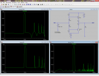
I'm simulating various circuits with LTSPICE, attaching a 1kHz sine wave to the input and looking at the FFT of the output voltage wave.

I've been using the default simulation command, "tran 10m", and was using magnitude of the distortion peaks to optimize the circuit.

The problem, and as far as I can determine this is a general effect for complimentary stages, is that the "tran 10m" (analyse the first 10 ms of simulation data) result is radically different than "tran 100m 90m" or "tran 1000m 990m" (analyzing 10 ms of data after 90ms and 900ms have elapsed, respectively). The distortion for the later data is markedly higher. I suggest they are too high to be realistic.

Any thoughts as to what's going on here?

(in image, temp.fft is 90ms, temp[1].fft is 0ms, and temp[2].fft is 900ms delay.)

 

[jcx]

the very 1st thing in using fft or .fourier Ltspice is to add the directive
.option plotwinsize=0
to your asc - Ltspice default applies data compression to the waveform that gives poor fft results - the .option statement turns off data compression

next it is good to give .tran a t_max_step_size that gives enough points in the sim - the sim time / ( 2 x # fft points ) is good to reduce interpolation artifacts, lots coarser time step/fewer points can be used but suspect the results

I like the Blackman window (fft dialog box) - reduces the truncation spectral spreading "noise floor" - of course always use a record time that fits an exact # of the fundamental periods

 

[rjm]

t_max_step_size was indeed the problem. With the longer total simulation times, the step interval was being automatically made coarser, which had a serious negative impact on the FFT quality.

Explicitly setting t_max_step_size to a sufficient small value so as to give ~1000 points in the sampling window made all FFT results look like the one obtained over 0-10 ms, independent of the total simulation time.

Thanks jcx, that saved me a bundle of trouble!

 

[IG81]

Doing a similar thing in AIM-Spice, I usually go with a measurement window after some time has elapsed on the circuit. As you found out, the trick is indeed to keep similar number of samples in the window, regardless of total simulation duration.

IG

 

[macboy]

It is also important that the plot contains a whole number of sine cycles so that it is DC balanced. Otherwise, the FFT will have a high noise floor that seems to slope down as frequency increases.

In order to easily change the frequency while maintaining the proper sample size and other parameters (like fourier frequency) I use a .param statement for the frequency. So my schematic will have these spice directives:

.option plotwinsize=0
.param Freq=5k
.tran 0 {20/freq} {1/freq} {.0001/freq}
.fourier {Freq} V(INPUT)
.fourier {Freq} V(OUTPUT)

The Input and output nodes of the amp are labelled INPUT and OUTPUT respectively.
By simply changing the Freq parameter, everything else changes automatically, so that the simulation runs for 21 cycles, saving and plotting the last 20 cycles, with a timestep giving 200000 points (why not?), and the fourier is computed for the correct frequency also.

 

[rjm]

@macboy

I believe that applying a window (Hamming, etc) to the data before proceeding with the FFT achieves the same result.