Still playing with Aksan's VPR. I don't find that negative coefficients are doing anything. I'm trying a Bessel array and not getting any difference with a -1 coefficient.
Graaf: short Bessel array. Yes, I agree that they are generally not useful. I do put them into programs as an easy check of whether the model appears to be working or not.
NC535: Thanks for more illustrations on Vituix. Still intending to learn it. Are there any off-the-shelf drivers for making generic systems?
Occasionally someone will post graphs of polars that you can use Vituix spl trace tool to capture but what seems to work well for this preliminary design exploration is to combine the published axial response from the driver's spec sheet with a baffle response in vituix diffraction tool The tool will generate a set of polars with the baffle direction, axial response and Sd piston directivity. With a waveguide on the ATH/ABEC/VACS you get a set of directivity files as well. On the ASR site, Klippel NFS directivity files are often posted. I got the files for KEF coax that way which is an interesting piece for the center of an array.
Agreed that Bessel arrays are not suited for lowering level of vertical reflections in domestic listening environments. They may be useful for horizontal use to increase SPL capability, although waveguides might be used to similar effect. If you have tall floor to ceiling arrays, the weighting becomes less important. But with shorter lines it can still be useful if vertical reflections are troublesome and you aren’t able to attack the problem with room treatment....From the perspective of lowering of the level of vertical reflections the short Bessel array looks as useless as expected, and the weighting of the long array does seem not worthy of the effort it takes, doesn't it?
They really are…mind boggling actually if you are used to measuring polar response of discrete tweeter or midrange arrays. The usual passive implementation with weightings (0.5, 1.0, 1.0, -1.0, 0.5) is just an approximation of the actual Bessel function values. If you use the actual values for 7 sources, pretty much all the ripples disappear in the far field polar; wrinkles will remain in the near field though.@bolserst that Bessel is surprisingly well behaved!


The other issue with Bessel arrays to be aware of is the phase response. Even though the magnitude of the response is nice and uniform, for a given frequency the phase response changes with angle, oscillating between +/-90deg. Similarly, for a give angle, you will see a phase response that changes with frequency. So the effective acoustic center is moving forward and backward with angle and frequency. How important that is to our listening experience might be debatable. But, this does make them difficult to cross over to drivers covering other frequency ranges. They pretty much have to be used as full range or tweeter arrays.


Last edited:
Thanks! 🙂Love the animations.
VBA = Visual Basic for Applications.I assume VBA means Visual Basic? I was looking into doing "for" loops in excel and the answer was always Visual Basic. Not sure I want to learn more languages but I would certainly like to see the results if you convert over to excel and VBA.
This can be accessed by key combination [Alt]+[F11] in Excel, Word, or Power Point.
Microsoft has ceased to support Visual Basic as a stand-alone development tool. However, it is my understand that they plan to continue to develop and support VBA. It is really handy to have ready access to plotting capability and portability of Excel. I’ll transfer over one of the simpler polar plotters to Excel and post as an example for you to look at how VBA can be used without much effort to loop, calculate and save results. I understand not wanting to waste brain cells on learning yet another language, but it is(pardon the pun), a rather basic language with not completely foreign syntax if you are coming from FORTRAN. Then again...maybe this is all OBE if VituixCAD does what you need.
There was an AES Convention paper from 1986 on finite line sources that contained similar plots....The next section of the paper shows the draw away curves. These would be a single tone (1k, 3.2 k, and 10k in figures 28, 29 and 30). All had a similar characteristic where they fell roughly 3 dB per distance doubling (as expected of a line source) and when through a periodic ripple. At some distance the ripple stops and the curve starts to fall at 6dB per distance doubling. This is described in figure 31 where the ripple appears to be the outer elements going in and out of phase (inner elements are largely uniform in distance) until the outermost elements are largely in phase with all the center elements and no more ripple can occur. This was a neat realization to me and I don't believe that anything had been published on this phenomenon previously.

The paper included quite a bit of theoretical background including derivation of the relationship between the 3dB/6dB breakpoint and listening distance/source length.
f = r*c/L^2 where:
f = frequency of breakpoint
r = listening distance
c = speed of sound
L = length of line source
The Acoustic Radiation of Line Sources of Finite Length
Authors: Lipshitz, Stanley P.; Vanderkooy, John
AES Convention: 81 (November 1986) Paper Number: 2417
Publication Date: November 1, 1986
https://www.aes.org/e-lib/browse.cfm?elib=5013
Among other plots, there was one showing that this same breakpoint formula defines the start of the -3dB slope in the frequency response for a given line length and listening distance.

Thanks for the L&R reference. I had not seen their paper before. Results look similar.
Mark Ureda of JBL had similar curves in his papers a few years after mine. (Great minds...)
Mark Ureda of JBL had similar curves in his papers a few years after mine. (Great minds...)
Now that we have a way of plotting out 23 element (or less) arrays with arbitrary weighting "profiles" we can look at the last section of the McIntosh paper that looked at improving the 16 element XRT24. Measurements to that point showed that floor to ceiling array were fairly invariant over a moderate standing to sitting height. But with mid length arrays (the 16 tweeter array was about 1.2 m in length) the standing to sitting variation was considerable. What height do you equalize for when the response is quite a bit different 0.5m up?
Below is the plot of both an unweighted (blue curve) vs a weighted (orange) of 16 elements. Weighting coefficients are 0.32, 0.32, 0.7, 0.7, 0.9, 0.9, 1.0, 1.0, 1.0, 1.0, 0.9, 0.9, 0.7, 0.7, 0.32, 0.32 . (Some zeros preceed and follow this to shrink my model from 23 tweets to 16.) Obviously for the blue curves the 16 coefficients are 1.0.

As you can see the weighted coefficients vertical directivity is considerably smoother and has lost the ripple. As adjacent frequencies were also smoothed the variation vs. frequency and vs. height was smoothed and the axis of EQ was less consequential.
No on axis sensitivity lost here (curves touch at 0 elevation height) but the blue curve has wider directivity, which seems odd as you would think that the weighting coefficients tend to shorten the effective length of the weighted array (from turning down outer elements).
Attached is the last of the AES paper. The curves shown above are the 3rd curve down in figure 36 (unweighted) and 37 (weighted). Note that the weighted curves are considerably cleaner vs frequency and also versus distance. I can't think of any good reason why a designer wouldn't follow this approach.
Below is the plot of both an unweighted (blue curve) vs a weighted (orange) of 16 elements. Weighting coefficients are 0.32, 0.32, 0.7, 0.7, 0.9, 0.9, 1.0, 1.0, 1.0, 1.0, 0.9, 0.9, 0.7, 0.7, 0.32, 0.32 . (Some zeros preceed and follow this to shrink my model from 23 tweets to 16.) Obviously for the blue curves the 16 coefficients are 1.0.
As you can see the weighted coefficients vertical directivity is considerably smoother and has lost the ripple. As adjacent frequencies were also smoothed the variation vs. frequency and vs. height was smoothed and the axis of EQ was less consequential.
No on axis sensitivity lost here (curves touch at 0 elevation height) but the blue curve has wider directivity, which seems odd as you would think that the weighting coefficients tend to shorten the effective length of the weighted array (from turning down outer elements).
Attached is the last of the AES paper. The curves shown above are the 3rd curve down in figure 36 (unweighted) and 37 (weighted). Note that the weighted curves are considerably cleaner vs frequency and also versus distance. I can't think of any good reason why a designer wouldn't follow this approach.
Attachments

Hear is the nearfield spreadsheet for you to play with. There is a tab for the 23 element array and a second tab with it calculating the 16 element array plotted above.
Put you own numbers in the "Weighting coefficients" line and see what you can come up with. Convert some first and last coefficients to zeros to shorten your array to any desired length. See how that impacts dispersion. All the yellow fields (element spacing, listening distance) are adjustable.
I know this approach only shows one frequency at a time but you get pretty good at seeing the trend as you adjust any particular variable. I typically calculate one variable setting, cut and paste the result line (far right line of the spreadsheet), change the variables and plot the recalc. A little slow but it works.
Attachments
Has anyone tried the spreadsheet? Note that you can use it to predict directivity of a continuous source such as electrostatic speaker, as long as you stay below the frequency of lobing. An electrostatic system could be given a weighting profile either by spreading the stator plates near the ends or by splitting the plates into zones with diminished drive near the ends.
Some researchers have shown the theoretical possibility ( some of you have linked excellent papers) but I don’t think any company but Quad have shown the engineering competency to tackle it.
Missed opportunity.
Some researchers have shown the theoretical possibility ( some of you have linked excellent papers) but I don’t think any company but Quad have shown the engineering competency to tackle it.
Missed opportunity.
Hi David:
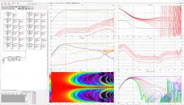
I tried the spreadsheet a little bit but I still prefer Vituix 🙂 . I modeled the 23 element array in Vituix, using TC9FD for the driver model. Your weights look pretty good. The orange trace in the middle graph is the in-room response with floor and ceiling reflections included. That dip at 200 hz goes away if the weights on the outer elements are replaced with shelf filters that shelve down to the weight. The vertical directivity in the mid range and treble is tall enough (the uppermost pink line in the vertical line chart is for 5 degrees) for seated height variations among seated listeners but not enough for both seated and standing listening. I haven't figured out how to fix that yet, at least not in a line array...
I have some other things going on that conflict with this thread but I remain very interested in it.
Attachments
I have something neat I came up with, inspired by this thread. A way to power taper an array passively, with a minimum of components. I'll post the article after work today.
Well, we have made the move from our Boston beach shack back to Austin. We split the drive up into 4 days drive with stops at relatives in Cleveland and Little Rock.
I came back just in time for the Austin City Limits outdoor concerts (next 2 weekends). All we can hear from our house is the bass. The arrays must be aimed away but are non-directional in the low frequencies (damned arrays!)
I have picked up the task again and continue to dabble withand learn Vituix. I've taken nc535's model (thanks!) and added lowpass filters to all sections but the central unit. I'm dabbling with progressively lower filters as you move from the middle (Its XA!) and have fair behaviour but still lobing from the central 3. You really do want a central cluster of physically tight dimensions, such as a small diameter tweeter between 2 mids. (Where did I hear that idea before...)
Anyhow, here is a look at it. I'll keep playing with it.
I've got a long way to go, and I don't even have any output to plot yet. But at least I can specify the array and locate the driver coordinates--that code takes a lot longer to develop than the ray tracing. My interest is for active two-way arrays with multiple amps and many channels of DSP, and I came around to seeing the benefit of modeling the DSP control for those arrays. The end goal is to be able to send commands to the array via Bluetooth BLE (from the .NET app) and at least get a rough feel for the room response from the model. The model will use both point source and "piston sources" for the drivers, a two-way crossover, shading and curvature.

That result from the 23 driver array @speaker dave posted is not that far off from what I have ended up with.
My array being a 25 driver array, using 4 filtered groups of 5 drivers and one unfiltered group of 5.
I wanted to find out if I could create a "better overall" performing array with filters than an unfiltered series/parallel array.
My focus has been on creating the smoothest directivity plot and an as wide as possible vertical "sweet area". To achieve this I used 'some' interference of the groups to keep/get the vertical "bundle" as wide as possible. It also meant I needed to keep the group of 5 drivers unfiltered on top. There still is lobing because of the spacing and yes, I've thought about adding a central smaller array or plannar to be able to get rid of that. In practice I just don't know if it will be worth it.
(as I'm having a lot of fun listening to this 'filtered' array)
Out in the (real) room the results are quite close to the predictions and that means I have a pretty large area (moving up/down and left/right) where the sound from both speakers is pretty much constant in SPL (after DSP correction).

(room settings: 4 dB damping for floor and ceiling, front and left wall turned off, dimensions according to my room and array)
While coming up with the above, which had unevenly divided driver groups due to sticking with 5 groups of 5 drivers, I did make a simulation of a slightly different arrangement. 24 drivers in a similar array with the driver at the listening height omitted:

(no EQ applied yet)
Slightly different goals here, getting the widest vertical bundle while trying to keep as close to the 3 dB/octave drop as possible.
As said, a hole in the 1 meter position waiting for a clever center solution.


Maybe I'll continue with this proposal if a clever center solution that fits within the "one driver" position exists.
My array being a 25 driver array, using 4 filtered groups of 5 drivers and one unfiltered group of 5.
I wanted to find out if I could create a "better overall" performing array with filters than an unfiltered series/parallel array.
My focus has been on creating the smoothest directivity plot and an as wide as possible vertical "sweet area". To achieve this I used 'some' interference of the groups to keep/get the vertical "bundle" as wide as possible. It also meant I needed to keep the group of 5 drivers unfiltered on top. There still is lobing because of the spacing and yes, I've thought about adding a central smaller array or plannar to be able to get rid of that. In practice I just don't know if it will be worth it.
(as I'm having a lot of fun listening to this 'filtered' array)
Out in the (real) room the results are quite close to the predictions and that means I have a pretty large area (moving up/down and left/right) where the sound from both speakers is pretty much constant in SPL (after DSP correction).
(room settings: 4 dB damping for floor and ceiling, front and left wall turned off, dimensions according to my room and array)
While coming up with the above, which had unevenly divided driver groups due to sticking with 5 groups of 5 drivers, I did make a simulation of a slightly different arrangement. 24 drivers in a similar array with the driver at the listening height omitted:
(no EQ applied yet)
Slightly different goals here, getting the widest vertical bundle while trying to keep as close to the 3 dB/octave drop as possible.
As said, a hole in the 1 meter position waiting for a clever center solution.
Maybe I'll continue with this proposal if a clever center solution that fits within the "one driver" position exists.
Great to see that you guys are coming up with a variety of solutions independently!
Just a couple of comments regarding the cluster spacing, especially of central elements and at high frequencies.
My array started with constant 80mm spacing as that was a good typical distance for either tweeters with larger mounting flanges or nominal 2 1/2 or 3 inch full range units.
This is not close enough to avoid some lobing at highest frequencies.
Even with strong rolloff outside the center element (with some possible compromise in high frequency power handling), a strong single lobe is evident around 5 kHz.

If i adjust the spacing of central elements to 40 mm the central directivity improves. There is a softer lobe pushed down to about 1 kHz and good uniformity to the edge of the green zone (about 10 to 15 dB down from the central peak and at a uniform angle of about 30 to 40 degrees.
Remember that this doesn't required that all elements are 40mm apart. My example has the central 7 at that spacing and then jumps to the previous 80 mm locations. We really just need the elements to be close until the outer units are rolled off enough for the wavelengths to relativly long compared to element spacing.
Ultimately this notion will lead to a log spaced concept with elements having upper cuttoff frequencies in proportion to element spacing and element spacing growing by a multiplier for each pair away from the middle. (Antenna people will be thinking of log periodic antennas at this point.)

We should probably contemplate what the design goal is here. I worry most about the direct sound and want to be able to stand and sit at a typical listening distance and hold the response to flat with a maximum level variation of, say, 2 dB. I definitely would want to be able to EQ the center axis to flat and see that hold (null free) over maybe +-20 degrees.
I would want to stay away from large peaks well off axis that might bounce off the floor or ceiling, once I had controlled the direct response. I don't think I would worry about the blue and pink level minor lobing seen in these plots as it is in the -30 dB level range.
Finally, just a look at turning off the central element. This seems like a messy approach with lots of lobing in the 5kHz and up region and on axis narrowing around 3 and 6 kHz. A gap in the middle of the element layout isn't good.

I think these Sims will always draw us back to a conclusion that we need a tight central cluster and then the array can spread out from there. Either a tweeter with two mids touching it or even three tweets in the center will add some complexity but will always improve the off axis, high frequency lobes.
Just a couple of comments regarding the cluster spacing, especially of central elements and at high frequencies.
My array started with constant 80mm spacing as that was a good typical distance for either tweeters with larger mounting flanges or nominal 2 1/2 or 3 inch full range units.
This is not close enough to avoid some lobing at highest frequencies.
Even with strong rolloff outside the center element (with some possible compromise in high frequency power handling), a strong single lobe is evident around 5 kHz.
If i adjust the spacing of central elements to 40 mm the central directivity improves. There is a softer lobe pushed down to about 1 kHz and good uniformity to the edge of the green zone (about 10 to 15 dB down from the central peak and at a uniform angle of about 30 to 40 degrees.
Remember that this doesn't required that all elements are 40mm apart. My example has the central 7 at that spacing and then jumps to the previous 80 mm locations. We really just need the elements to be close until the outer units are rolled off enough for the wavelengths to relativly long compared to element spacing.
Ultimately this notion will lead to a log spaced concept with elements having upper cuttoff frequencies in proportion to element spacing and element spacing growing by a multiplier for each pair away from the middle. (Antenna people will be thinking of log periodic antennas at this point.)
We should probably contemplate what the design goal is here. I worry most about the direct sound and want to be able to stand and sit at a typical listening distance and hold the response to flat with a maximum level variation of, say, 2 dB. I definitely would want to be able to EQ the center axis to flat and see that hold (null free) over maybe +-20 degrees.
I would want to stay away from large peaks well off axis that might bounce off the floor or ceiling, once I had controlled the direct response. I don't think I would worry about the blue and pink level minor lobing seen in these plots as it is in the -30 dB level range.
Finally, just a look at turning off the central element. This seems like a messy approach with lots of lobing in the 5kHz and up region and on axis narrowing around 3 and 6 kHz. A gap in the middle of the element layout isn't good.
I think these Sims will always draw us back to a conclusion that we need a tight central cluster and then the array can spread out from there. Either a tweeter with two mids touching it or even three tweets in the center will add some complexity but will always improve the off axis, high frequency lobes.
The program in the link still has a way to go, but it's fun to play with in its current state. You can use the mouse to rotate the 3D chart, which makes it easier to understand the response vs frequency and vertical angle. You can change the number of drivers, adjust shading and curvature, and turn on or off the piston model (the piston model sums the response from the all the white dots on the driver, instead of just using the center points). There is no smoothing in the chart, so it will look a bit ragged where there is steep cancellation. There are 61 angles, from -30 to 30, and 125 log-spaced frequencies.
Only the mid array is working, and the updates are slow because the code isn't multi-threaded (yet). No crossover, yet, either, but I've got all the code for the crossovers and multi-threading elsewhere in the code. The code is part of a larger program that will allow updating the line array DSP shading and curvature and frequency response in real time via Bluetooth BLE.
Other notes: the "Spacing" parameter is the space between the drivers, not the center-to-center spacing, and all measurements are in feet or inches
Installation hint: you will no doubt get errors trying to download the code because my site isn't using https, and Windows will report the code as "unsafe". But it's just a .NET program that is perfectly safe.
Caveat: I had verified that the 2D code was generating the same response data as Dave's most recent spreadsheet for fixed frequencies, but I haven't spent much time trying to verify the 3D version with frequency as a variable.
These screen captures are front and side views of the 23-driver array with no shading or curvature at 12 feet away.
I really like the Chart Director graphing tools. The chart component is easy to use, and it has a lot of nice features, including the ability to programmatically set the elevation and rotation angles and sample code for the mouse handlers. The developer license is only $99, which I will probably buy, but the distribution license is $500, and I'm not committed enough to this project to pay for that yet. Without the license, the product works fine, but there is a yellow bar at the bottom of the chart that reminds you that the product is unregistered.


I really like the Chart Director graphing tools. The chart component is easy to use, and it has a lot of nice features, including the ability to programmatically set the elevation and rotation angles and sample code for the mouse handlers. The developer license is only $99, which I will probably buy, but the distribution license is $500, and I'm not committed enough to this project to pay for that yet. Without the license, the product works fine, but there is a yellow bar at the bottom of the chart that reminds you that the product is unregistered.
Hi Neil,
Nice progress on your array simulator. I played with some different options and the results seem very plausible. A straight 5 element array gives the 3 lobes between aliases that look as expected (I also typically use a Bessel array as a common check, assuming you can put in positive and negative multipliers).
I caught that your spacing was element edge to element edge. I would recommend you make it center to center as it is often useful to "double the spacing" to see the effect and that would be easiest if the number represented the center to center span.
It would be nice to be able to use the data and pull out a 2D slice, either polar response for one frequency or frequency response for one angle.
I like the windowing portion. What is log shading? It gives a smooth result.
David
I mentioned at one point that antenna people are dealing with a lot of the same issues as speaker array designers. I was looking through some antenna articles and found a few interesting papers that should be food for thought.
Here is an article on designing ultrasound transducers that are lobe free.
https://www.nature.com/articles/s41598-019-50317-7
In the diagram he shows a transducer with a number of elements with a circular delay to focus at a point. As it is a finite aperture it shows typical side lobes (would appear to be ringing if it were a time waveform). This is the blue curve. He then shows a second delay profile (orange curve) that is nulled at its very center and then rings similarly to the first profile except the ringing is opposite phase . The two are then added to give a central peak as before but with all the ringing cancelled. This would give a sharper ultrasound image.

In spite of this being an ultrasound application the approach could be applied to a loudspeaker array.
Nice article here about TV antennas. I wondered why the elements were angled forward. The text explains that it increases front to back gain and also diminishes all lobes!
https://worldradiohistory.com/Archive-Electronics-World/60s/1966/Electronics-World-1966-02.pdf
(Starts on page 45)

This should work for a speaker array as well. Something that we need to model.
Note that the elements vary in length. This is part of a commonly used "log periodic" form. With a log periodic, each element is an active dipole (not a reflector or director) and both the spacing from element to element and the element length are large at one end and shrink by a constant percentage for every smaller element (length and spacing is a logarithmic progression).
Heck, Lafayette Radio would sell you one for $8.79.

Log spaced speaker arrays would be anything similar to the Snell XA models with progressivly expanding element spacing for lower frequency range elements. The approach was also used by us in Bose sound bars.
I don't know how this one works but the name alone: "UltraHorn" makes you want it. Another lobe free design.
https://rfelements.com/products/ultrahorn/ultrahorn-directional-antennas/overview

All for now.
David
Here is an article on designing ultrasound transducers that are lobe free.
https://www.nature.com/articles/s41598-019-50317-7
In the diagram he shows a transducer with a number of elements with a circular delay to focus at a point. As it is a finite aperture it shows typical side lobes (would appear to be ringing if it were a time waveform). This is the blue curve. He then shows a second delay profile (orange curve) that is nulled at its very center and then rings similarly to the first profile except the ringing is opposite phase . The two are then added to give a central peak as before but with all the ringing cancelled. This would give a sharper ultrasound image.
In spite of this being an ultrasound application the approach could be applied to a loudspeaker array.
Nice article here about TV antennas. I wondered why the elements were angled forward. The text explains that it increases front to back gain and also diminishes all lobes!
https://worldradiohistory.com/Archive-Electronics-World/60s/1966/Electronics-World-1966-02.pdf
(Starts on page 45)
This should work for a speaker array as well. Something that we need to model.
Note that the elements vary in length. This is part of a commonly used "log periodic" form. With a log periodic, each element is an active dipole (not a reflector or director) and both the spacing from element to element and the element length are large at one end and shrink by a constant percentage for every smaller element (length and spacing is a logarithmic progression).
Heck, Lafayette Radio would sell you one for $8.79.
Log spaced speaker arrays would be anything similar to the Snell XA models with progressivly expanding element spacing for lower frequency range elements. The approach was also used by us in Bose sound bars.
I don't know how this one works but the name alone: "UltraHorn" makes you want it. Another lobe free design.
https://rfelements.com/products/ultrahorn/ultrahorn-directional-antennas/overview
All for now.
David
- Home
- Loudspeakers
- Multi-Way
- Line arrays. Understanding their behavior through simple modeling