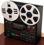
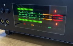
The analog level meter has been designed for use as a recording level meter for a reel to reel tape recorder. But it can also be used as a standalone device. The LED bar can contain up to 50 elements per channel. To reduce the level of interference, static indication is used. A feature of the meter is fully digital signal processing. That allows you to make the meter metrologically accurate, with an exact match of the dynamic characteristics. All parameters are programmed using special software on a computer.
Each meter channel contains two signal processing branches, the readings of the first one are displayed as a bar, the second - as a dot. This can be used to display two values, such as average + quasi-peak, or quasi-peak + true peak. For each of the branches, you can individually set the gain, integration time, response time, decay time, hold time, fall time, peak hold time, peak fall time. The scale type is set by assigning an individual threshold level to each LED with an accuracy of 0.01 dB. This allows you to build a linear, logarithmic, S-shaped with a stretch near 0 dB and other scales. A set of all parameters, including the scale type, is stored in EEPROM as a preset. There can be 4 different presets in total. They can be selected with the control button. The second button can turn on the indication of statistics of maximum levels, as well as reset it.
Here we will talk about how simple things can be made difficult 🙂
Block diagram
The block diagram of the level meter is shown in the figure below. This diagram shows one stereo channel of the meter. The input signal is fed to a differential amplifier implemented on an op-amp (Meter50_v4_sch.pdf). It performs two tasks: it shifts the signal by half the ADC scale and allows you to implement a balanced input. The signal shift is necessary because the built-in ADC is unipolar, its input range is from 0 to the reference voltage. A balanced input is desirable even if the signal source is single ended. It allows you to take the signal relative to "analogue" ground and eliminate the interference present on the ground of the meter circuit. If the level meter is made as a separate device, then balanced inputs with XLR connectors can be implemented.

All signal processing is done digitally by the STM32F100/103 microcontroller. To avoid the use of an anti-alias filter at the ADC input, as well as to be able to register short signal peaks, the sampling frequency was chosen quite high - 96 kHz. With DMA, ADC samples are stored in a buffer in RAM. When half of the array is ready, an interrupt occurs, the data is read and processed.
DC removal filter
The first operation on digital data is to remove the DC component from the signal. This must be done before the signal is sent to the detector. With a meter dynamic range of about 60 dB, even such a small DC component as 0.1% of the ADC scale can be equal in magnitude to the useful signal and distort it.
Detector
Next, a full-wave rectification of the signal is performed. This is the easiest part of processing. When the DC component is removed from the signal, the task is to calculate the absolute value.
Filters
Next are several filters that define the dynamic characteristics of the meter.
Integration time
To obtain a given integration time, the detector output must be smoothed with a filter. The smoothing filter is not a simple low-pass filter, but a more complex filter with different charge and discharge time constants. The charge must be fast to provide the specified meter integration time. And the discharge must occur slowly to provide a given return time, which is much longer. Therefore, the integration time filter is turned on only when the signal rises; when the signal decreases, it is kept at the same level. A separate filter is used for signal decay.
The difference filter equation has the following form:
y( n ) = y(n-1) + A*(x( n ) - y(n-1)), where A = 0.0083 for Fs = 96 kHz
A 32-bit accumulator is used to obtain the required calculation accuracy. Filter coefficients are 16-bit unsigned. They are defined as A = 65536 / 96000 / tau.
Each meter channel contains two signal processing branches, the readings of the first one are displayed as a bar, the second - as a dot. This can be used to display two values, such as average + quasi-peak, or quasi-peak + true peak. For each of the branches, you can individually set the gain, integration time, response time, decay time, hold time, fall time, peak hold time, peak fall time. The scale type is set by assigning an individual threshold level to each LED with an accuracy of 0.01 dB. This allows you to build a linear, logarithmic, S-shaped with a stretch near 0 dB and other scales. A set of all parameters, including the scale type, is stored in EEPROM as a preset. There can be 4 different presets in total. They can be selected with the control button. The second button can turn on the indication of statistics of maximum levels, as well as reset it.
Here we will talk about how simple things can be made difficult 🙂
Block diagram
The block diagram of the level meter is shown in the figure below. This diagram shows one stereo channel of the meter. The input signal is fed to a differential amplifier implemented on an op-amp (Meter50_v4_sch.pdf). It performs two tasks: it shifts the signal by half the ADC scale and allows you to implement a balanced input. The signal shift is necessary because the built-in ADC is unipolar, its input range is from 0 to the reference voltage. A balanced input is desirable even if the signal source is single ended. It allows you to take the signal relative to "analogue" ground and eliminate the interference present on the ground of the meter circuit. If the level meter is made as a separate device, then balanced inputs with XLR connectors can be implemented.
All signal processing is done digitally by the STM32F100/103 microcontroller. To avoid the use of an anti-alias filter at the ADC input, as well as to be able to register short signal peaks, the sampling frequency was chosen quite high - 96 kHz. With DMA, ADC samples are stored in a buffer in RAM. When half of the array is ready, an interrupt occurs, the data is read and processed.
DC removal filter
The first operation on digital data is to remove the DC component from the signal. This must be done before the signal is sent to the detector. With a meter dynamic range of about 60 dB, even such a small DC component as 0.1% of the ADC scale can be equal in magnitude to the useful signal and distort it.
The simplest filter that suppresses the DC component is the differentiator. It has one zero at zero frequency. The DC gain is zero (as required), and as the frequency increases, the gain increases. For a discrete implementation of the differentiator, its difference equation has the following form:
y( n ) = x( n ) – x(n-1)
In fact, this is the simplest FIR filter. When implementing, it must be taken into account that the output value must have a width of at least 1 bit more than the input value. Since the input signal in theory in one cycle can change to the full scale. Increasing the gain with increasing frequency is not satisfactory, since the gain will change in the operating frequency range. Instead, you need to get a linear frequency response above a certain cutoff frequency. Obviously, this requires adding a pole at the desired cutoff frequency. This can be done by connecting the differentiator and the 1st order low-pass filter in series. The overall frequency response will have the desired form. Such a 1st-order low-pass filter in such applications is often called a "leaky integrator". Because in the analog version, such an integrator is implemented by adding a resistor in parallel with the capacitance, through which it will slowly discharge. For a discrete implementation, the difference equation of an ideal integrator is given below:
y( n ) = y(n-1) + x( n )
To add a leakage, you need to multiply the accumulated value by some coefficient less than one:
y( n ) = A*y(n-1) + x( n ), 0 < A < 1
This is the simplest IIR low pass filter. The name "leaky integrator" is used to indicate that this filter is applied in a somewhat unusual way - the operating frequency band lies in the stopband.
The cutoff frequency here should be chosen low compared to the sampling rate, which means that the A coefficient should be close to unity. The cutoff frequency can be calculated using the equation:
f = (1 - A)*Fs/2*pi, or A = 1 – 2*pi*f/Fs, where Fs is the sampling frequency.
The general difference equation for the filter will look like this:
y( n ) = x( n ) – x(n-1) + A*y(n-1)
In fact, this is a first-order IIR high-pass filter. It is equivalent to a differentiating RC chain. Such a filter has one zero and one pole. If you show them on the z-plane, then zero will lie at the point z=1, and a little to the left of it on the axis there will be a pole.
The audio bandwidth starts at 20 Hz. But it is desirable to make the cutoff frequency lower so that a noticeable phase shift does not appear in the audio band. This filter is not phase-linear, so signal components of different frequencies will be delayed for different times. The result of their addition will give a different waveform, the peak level will be incorrect. There are phase-linear FIR high-pass filters, but they require a lot of computing resources to obtain good linearity of the frequency response in the passband at a low cutoff frequency. There is a filter option for removing DC component based on MAF (moving average filter). It doesn't use much computational resources, but it does require a lot of memory to get a high sample rate to cutoff frequency ratio.
In this case, the requirements for the filter are not very strict. It is necessary to remove the DC voltage, which can only change very slowly (for example, due to the temperature drift of the op-amp). A significant part of the compensated bias is generally constant, as it is associated with the error of the bias voltage divider. Therefore, you can simply make the cutoff frequency lower, while minimizing the phase shift. A cutoff frequency of about 5 Hz would be a good choice. The phase shift at a frequency of 20 Hz will be about 17 degrees, which can be considered acceptable.
When implementing a filter in integer arithmetic, one must take care of the ranges of numbers at all stages of the calculation so that overflow does not occur. The leaky integrator and differentiator can be connected in any order. But to avoid overflow, the differentiator should be included first.
Another problem, more complex, is related to rounding errors. For a filter cutoff frequency of 5 Hz at a sampling rate of 96 kHz, the value of the coefficient A = 0.999673. To carry out calculations with such a coefficient with good accuracy, it is required to increase the bit depth. The reverse transition will be a quantization with a larger step, which leads to the appearance of an error, or quantization noise. As a result of such an error in the filter, a parasitic constant component may appear at the output, which is even greater than the one that is suppressed. This error may cause the filter to fail. As a practical test has shown, the filter does not actually work without requantization error correction.
In this case, the ADC is 12-bit, the samples are placed in 16-bit signed integers. Some margin is needed here to protect against overflow. Multiplication is done in 32-bit format. Then, when moving from a 32-bit intermediate result to a 16-bit result, a quantization error will occur. In one of the publications it is proposed to add a quantization noise spectrum shaper to the filter by introducing error feedback. The implementation of this method is very simple. I made my own implementation which uses the same error correction principle.
static const double POLE = 0.999673;
static const int32_t A = (int32_t)(UINT16_MAX * POLE);
static int32_t acc = 0;
static int16_t xx = 0;
static int16_t yy = 0;
x = Input;
acc = LO_W(acc) + A * yy;
yy = x - xx + HI_W(acc);
xx = x;
Output = yy;
Quantization occurs by discarding the lower half of the 32-bit number. The discarded value is the quantization error. The original number is signed, but the error is always negative. For example, if the least significant bits of a positive number are replaced with zeros, the number will decrease, and some positive number will have to be added to correct the error. If the least significant bits of a negative number are replaced by zeros, the number will become large in absolute value, while remaining negative. This means that in order to correct the error, you will again need to add some positive number. Therefore, the error can be extracted from the original 32-bit number by simply zeroing its high half along with the sign bit.
Detector
Next, a full-wave rectification of the signal is performed. This is the easiest part of processing. When the DC component is removed from the signal, the task is to calculate the absolute value.
Filters
Next are several filters that define the dynamic characteristics of the meter.
The main characteristics of level meters are integration time and return time. The integration time determines how quickly the meter reacts to changes in signal level. If the integration time is large (about 300 ms), the so-called VU-meter is obtained. Such a meter will not respond to short signal peaks that can overload the recording path. When pointer instruments were used as the indication device, the integration time could not be made small due to the inertia of the moving system. Therefore, often the VU-meter was combined with a faster LED peak indicator. The use of high-speed information display devices, such as gas discharge tubes or LEDs, removed the problem of obtaining short integration times and made it possible to build peak or quasi-peak meters.
Most often, quasi-peak level meters are used to measure the signal level in audio paths. Unlike true peak meters, which in theory have zero integration time, for quasi-peak meters this time is defined by the standards. It would seem that it is necessary to achieve the minimum possible integration time so that the indicator can register the shortest signal peaks without overloading the path. This approach is used in digital paths, where even a short-term overload leads to undesirable consequences. For analog magnetic recording, a short overload may not be audible at all. If you want to completely eliminate the overload at the peaks of the signal, you will have to reduce the average recording level, which will lead to a more audible problem - a decrease in the signal-to-noise ratio. Therefore, for analog magnetic recording, it makes sense to choose some optimal value for the integration time of the level meter so that it allows short-term overloads.
The integration time for quasi-peak meters is defined by IEC 60268-10 as "...the duration of a burst of sinusoidal voltage of 5000 Hz at reference level which results in an indication 2 dB below reference indication". This standard defines an integration time value of 5 ms for quasi-peak meters.
The integration time is not numerically equal to the charging time constant of the smoothing RC circuit. If an RC circuit with a charge time constant of 5 ms is installed at the output of the peak detector, then the level of -2 dB (about 0.8) will be reached in about 20 ms. To reach -2dB in 5ms, the charging time constant of the RC circuit would need to be around 1.25ms. Thus, the integration time is approximately 4 tau RC circuit.
In addition to the integration time, quasi-peak meters have a return time that is much longer. This time determines how fast the reading will fall after the signal is removed. If this time is made small (for example, equal to the integration time), then the indicator readings will change too quickly, making them difficult to read. For VU meters, such a problem did not arise due to their low speed, one time constant could be dispensed with. In high-speed quasi-peak meters, it is necessary to artificially slow down the fall in readings so that the operator can read the information.
The return time determines how quickly the meter reading will fall by 20 dB after the signal is removed. It is also not equal to the discharge time constant of the RC circuit, but is approximately 2.3 tau. The return time value is also set by the standards. It differs for indicators of different purposes. For indicators of the first type, which serve to check the signal level during its operational adjustment (this is just the case of adjusting the recording level in a tape recorder), the return time should be 1.7±0.3 sec. Accordingly, the discharge time constant of the RC circuit should be approximately 740 ms.
Level meters have another dynamic characteristic - response time. It may not be entirely clear. For inertialess devices, ballistics is artificially formed, similar to pointer devices. Increasing the response time in this case should not increase the integration time of the meter. The short signal pulses should still display correctly. To do this, the detector must "wait" until the reading reaches the measured value, and only then start the fall. In amateur designs of quasi-peak meters, with a fast increase in the signal level, the bar immediately jumps from one length to another. This is not the case with professional quasi-peak meters, because the increase in response time has a positive effect on the perception of readings by the operator. In VU meters, this is also not the case, there the smoothness of movement is obtained due to the large integration time. The response time is defined as the interval from the moment the test tone burst begins until the reading reaches -1 dB.
Integration time
To obtain a given integration time, the detector output must be smoothed with a filter. The smoothing filter is not a simple low-pass filter, but a more complex filter with different charge and discharge time constants. The charge must be fast to provide the specified meter integration time. And the discharge must occur slowly to provide a given return time, which is much longer. Therefore, the integration time filter is turned on only when the signal rises; when the signal decreases, it is kept at the same level. A separate filter is used for signal decay.
The difference filter equation has the following form:
y( n ) = y(n-1) + A*(x( n ) - y(n-1)), where A = 0.0083 for Fs = 96 kHz
A 32-bit accumulator is used to obtain the required calculation accuracy. Filter coefficients are 16-bit unsigned. They are defined as A = 65536 / 96000 / tau.
Attachments
-
Firmware.zip211.7 KB · Views: 128
-
Mask.zip92.8 KB · Views: 99
-
Pcb.zip537.9 KB · Views: 105
-
 mech.jpg84.6 KB · Views: 147
 -
 pcb_pro.jpg159.8 KB · Views: 165
 -
 pcb_ind.jpg233.9 KB · Views: 163
 -
Meter50_v4_pcb.pdf276 KB · Views: 127
-
Meter50_v4_sch.pdf351.9 KB · Views: 172
-
 01_r-r_deck.jpg142.6 KB · Views: 161
Last edited:

"Slow" domain
To obtain a return time of 1.7 seconds, a filter time constant of approximately 740 ms is needed. This is too long to process in the 96 kHz domain. Therefore, further processing is done in the "slow" domain. The reduced sampling rate is formed as the frequency of filling the halves of arrays of 256 points each with ADC data, i.e. 96000 / 256 = 375 Hz. This is quite a reasonable sampling rate for this filter, for 740 ms the filter coefficient is equal to 0.0036, which is quite an acceptable value.
Scaling
Processing in the "slow" domain begins with signal scaling, which is necessary to equalize the indications of the quasi-peak and peak levels on a stationary signal. The output 11-bit code of the previous filters is multiplied by the scaling factor. The output is a maximum code of 10000, it is this range that is used in the dB conversion table. After multiplication, the code is limited to about 10% above the maximum code for the dB table. At the maximum value of the coefficient, the gain is 32 (approximately +30 dB). You can use this gain to shift the scale when you need to measure small signals more accurately.
Response time
To form the response time, an IIR filter is used, which operates in the "slow" domain. The output code of this filter is directly related to the meter reading. A 32-bit accumulator is used to obtain the required calculation accuracy. As with the integration time filter, this filter only works when the signal is rising. Filter coefficient 16-bit unsigned. It is defined as A = 65536 / 375 / tau.
Decay time
It was said above that the integration time filter works only when the signal rises. It can only increase the output code. For signal decay, a special filter is used, which acts on the integration time filter accumulator. It only turns on after the response time has elapsed. Because the signal decays slowly, this filter operates in the "slow" domain. Filter coefficient 16-bit unsigned. It is defined as A = 65536 / 375 / tau.
Hold time
Decreasing the integration time filter accumulator code does not mean that the meter reading is decreasing. The readings are associated with the response time filters and may have some hold time where the reading remains unchanged after the peak of the signal. This can be used both to hold peak values and to eliminate fast flickering of bar segments. The hold time is set using a special coefficient, which is calculated by the formula A = 375 * t_hold. If you set a zero value, the readings will not be held, and immediately after the end of the response time, the return will begin.
Fall time
When the hold time ends, the meter begins to return. For this, a falling time filter is used. This filter acts on the response time filter accumulator. The filter works in the "slow" domain. Filter coefficient 16-bit unsigned. It is defined as A = 65536 / 375 / tau. This time constant determines the meter's fall time.
A separate fall time implementation for the response filter allows for reduced decay time for the integration filter, which reduces the effect of peak-to-peak time on the meter reading. There is usually such an influence - if the signal peaks at the meter input are repeated more often, then the readings increase (even when the magnitude of these peaks remains unchanged). This is due to the fact that by the time the next peak begins, the integration filter has not had time to completely "discharge", a new increase in its output signal starts from a higher initial value. As a result, it will be able to achieve a higher value than in the case of rarely repeated peaks.
When a filter has different integration and return time constants, the magnitude of the output signal will depend on the ratio of these times. If these times were the same, it would be a simple averaging filter, the output of which would be the average value of the signal (for a sine, this is 0.637 of the peak value). If you increase the return time in relation to the integration time, the output signal will increase and in the limit will become equal to the peak value of the input signal, when the ratio of the return time to the integration time becomes infinite. The situation is similar for a conventional analog detector with a smoothing filter with different charge and discharge time constants. Therefore, if the ratio of the time constants changes, the calibration of the meter will be violated, which requires correction using scaling factors.
Maximum values
In each processing branch, the maximum (peak) value of the measured signal can be stored and held for some time. For storage, a special accumulator of the maximum value is used. When the hold time ends, the return begins. The holding time and the return time for the maximum values are given by separate coefficients. As a result, the meter allows you to get 4 different output values, which helps to implement various display modes.
Statistics
In addition to the accumulators of peak values, there are also accumulators that are used to accumulate statistics. When the meter is running, the values in these accumulators can only increase. There is no return here. Resetting statistics is done manually.
Special note on VU
The flexible setting of the coefficients makes it possible to implement various types of meters. Separately, it should be said about the VU meter, which used to be the most common. To be able to compare readings with old devices, it would be useful to have such a mode. For the VU meter, the standard defines the same charge and discharge time constants of 300 ms. At first glance, it seems that this problem is solved simply - it is enough to choose the necessary integration and return time constants. However, for VU meters, the standard defines the 300 ms time differently: this is the time during which the reading reaches 99% of the steady state value, and then an overshoot from 1 to 1.5% follows. Previously, this was provided by a mechanical movable system of a pointer measuring device. To implement this electrically, a 2nd order low-pass filter with a cutoff frequency of 2.1 Hz and a quality factor of 0.62 is required. This is something between Bessel and Butterworth filters. Here, such a filter has not yet been implemented. But even with a 1st order filter, you can choose a transient response, on average, similar to the standard one for VU. This will require tau approximately 130 ms. Then only 90% will be reached in 300 ms, but in general the behavior of the meter will be very close to VU. In this case, it is not entirely correct to state that the meter supports VU mode, but in practice the difference in readings will be insignificant.
LED scale table
The result of digital processing of the input signal is numbers in the range from 0 to 10000. These numbers are updated with a sampling rate of the "slow" domain of 375 Hz. They represent the magnitude of the signal on a linear scale. The scale of the meter is most often made non-linear. It can be logarithmic, or even more complex, such as an S-shape with a stretch around 0 dB.
A table is used to set an arbitrary scale. It is common for two stereo channels and contains the number of elements equal to the number of LEDs in the bar. Each value in the table corresponds to a threshold for one segment. It is specified in dB with a resolution of 0.01 dB. The values in the table must be monotonic. The last element of the table is the maximum level. The difference between the maximum and minimum levels can be up to 80 dB. All levels below -80 dB are considered minus infinity. This level can be set for the first segment of the bar so that it is constantly lit.
To fill the table, there are special tools in the control program on the PC. The user can easily create their own scales, which are loaded into the meter via any USB-TTL adapter. They are stored as presets in a 24C16 type EEPROM chip. You can switch presets using jumpers or a button. Through the same port, it is possible to update the firmware of the microcontroller if the power is turned on with the BOOT jumper installed.
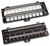
LED display
The LED bars are connected to the outputs of shift registers 74HC595, which are included in the chain and loaded via the SPI port. The hardware SPI of the STM32 microcontroller is used.
In addition to the LED bars, the meter contains stencils that are illuminated by LEDs. They can be used to indicate various operating modes. These LEDs can be turned on or off as specified in the presets. You can also control them from external signals connected through a special connector.
Brightness control
To equalize the brightness of the LED bars, as well as the scale and stencils, a separate brightness adjustment is required. It can be done in software or with pots. Software adjustment can use PWM or built-in DACs. For smoothing PWM, a 3rd order low-pass filter, performed on an op-amp, is used. From its output, the control voltage is fed to the adjustable stabilizers LM1117. As experience has shown, the use of PWM is undesirable due to the increase in the level of interference. The latest version uses pots.
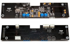
Printed boards
The meter consists of two printed circuit boards - an indication board and a processor board. The boards are connected to each other using connectors. When LED bars of different colors are used, then it is necessary to select limiting resistors for each color in advance so that the visual brightness is the same. The circuit diagram shows approximate values, with other types of bars they may be different. A similar situation with individual LEDs.
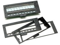
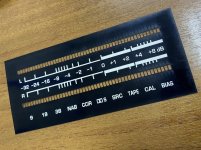
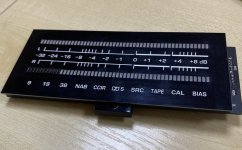
A diffuser in the form of a multilayer structure made of sheet plastic is installed on top of the indication printed board. With the help of laser cutting, parts are made, which are then assembled in a stack and glued together. A scale mask is installed on top, which is made using photo printing or laser engraving of thin two-layer plastic Rowmark LaserLIGHTS S61 (black / white). Drawing details and mask can be downloaded in the archive (Mask.zip).

Service software
The service software allows you to set the parameters of the meter, create new scales, and can also display the indicator readings on the computer screen. The view of the main program window is shown in the figure. All controls are intuitive and have hints. To fill the scale table, there is interpolation of the selected range of table cells: the cells are filled with values with a constant step, which is calculated from the last selected cells.
Default presets
Preset 1 - standard quasi-peak meter, integration time 5 ms, response time 100 ms, hold time 20 ms, fall time 1700 ms. Dots operates as a true peak meter, integration time 0 ms, response time 100 ms, hold time 1000 ms, fall time 600 ms.
Preset 2 - standard quasi-peak meter, integration time 5 ms, response time 100 ms, hold time 20 ms, fall time 1700 ms. Dots represent maximum bar values, hold time 1000ms, flyback time 600ms.
Preset 3 - simulation of the standard level meter of my reel-to-reel tape recorder, integration tau 12 ms (the time constant of the RC circuit is about 6 ms and a half-wave rectifier), return tau 1500 ms. The dot is not used.
Preset 4 - simulation of a Dorrough 40-A2 meter, integration and return tau 300 ms. The dot operates as a true peak meter, integration time 0 ms, response tau 10 ms, hold time 25 ms, fall tau 300 ms. Additionally, the peaks are held by one more dot, the hold time is 2000 ms, there is no reverse motion.
More info, video1, video2, video3.
To obtain a return time of 1.7 seconds, a filter time constant of approximately 740 ms is needed. This is too long to process in the 96 kHz domain. Therefore, further processing is done in the "slow" domain. The reduced sampling rate is formed as the frequency of filling the halves of arrays of 256 points each with ADC data, i.e. 96000 / 256 = 375 Hz. This is quite a reasonable sampling rate for this filter, for 740 ms the filter coefficient is equal to 0.0036, which is quite an acceptable value.
Scaling
Processing in the "slow" domain begins with signal scaling, which is necessary to equalize the indications of the quasi-peak and peak levels on a stationary signal. The output 11-bit code of the previous filters is multiplied by the scaling factor. The output is a maximum code of 10000, it is this range that is used in the dB conversion table. After multiplication, the code is limited to about 10% above the maximum code for the dB table. At the maximum value of the coefficient, the gain is 32 (approximately +30 dB). You can use this gain to shift the scale when you need to measure small signals more accurately.
Response time
To form the response time, an IIR filter is used, which operates in the "slow" domain. The output code of this filter is directly related to the meter reading. A 32-bit accumulator is used to obtain the required calculation accuracy. As with the integration time filter, this filter only works when the signal is rising. Filter coefficient 16-bit unsigned. It is defined as A = 65536 / 375 / tau.
Decay time
It was said above that the integration time filter works only when the signal rises. It can only increase the output code. For signal decay, a special filter is used, which acts on the integration time filter accumulator. It only turns on after the response time has elapsed. Because the signal decays slowly, this filter operates in the "slow" domain. Filter coefficient 16-bit unsigned. It is defined as A = 65536 / 375 / tau.
Hold time
Decreasing the integration time filter accumulator code does not mean that the meter reading is decreasing. The readings are associated with the response time filters and may have some hold time where the reading remains unchanged after the peak of the signal. This can be used both to hold peak values and to eliminate fast flickering of bar segments. The hold time is set using a special coefficient, which is calculated by the formula A = 375 * t_hold. If you set a zero value, the readings will not be held, and immediately after the end of the response time, the return will begin.
Fall time
When the hold time ends, the meter begins to return. For this, a falling time filter is used. This filter acts on the response time filter accumulator. The filter works in the "slow" domain. Filter coefficient 16-bit unsigned. It is defined as A = 65536 / 375 / tau. This time constant determines the meter's fall time.
A separate fall time implementation for the response filter allows for reduced decay time for the integration filter, which reduces the effect of peak-to-peak time on the meter reading. There is usually such an influence - if the signal peaks at the meter input are repeated more often, then the readings increase (even when the magnitude of these peaks remains unchanged). This is due to the fact that by the time the next peak begins, the integration filter has not had time to completely "discharge", a new increase in its output signal starts from a higher initial value. As a result, it will be able to achieve a higher value than in the case of rarely repeated peaks.
When a filter has different integration and return time constants, the magnitude of the output signal will depend on the ratio of these times. If these times were the same, it would be a simple averaging filter, the output of which would be the average value of the signal (for a sine, this is 0.637 of the peak value). If you increase the return time in relation to the integration time, the output signal will increase and in the limit will become equal to the peak value of the input signal, when the ratio of the return time to the integration time becomes infinite. The situation is similar for a conventional analog detector with a smoothing filter with different charge and discharge time constants. Therefore, if the ratio of the time constants changes, the calibration of the meter will be violated, which requires correction using scaling factors.
Maximum values
In each processing branch, the maximum (peak) value of the measured signal can be stored and held for some time. For storage, a special accumulator of the maximum value is used. When the hold time ends, the return begins. The holding time and the return time for the maximum values are given by separate coefficients. As a result, the meter allows you to get 4 different output values, which helps to implement various display modes.
Statistics
In addition to the accumulators of peak values, there are also accumulators that are used to accumulate statistics. When the meter is running, the values in these accumulators can only increase. There is no return here. Resetting statistics is done manually.
Special note on VU
The flexible setting of the coefficients makes it possible to implement various types of meters. Separately, it should be said about the VU meter, which used to be the most common. To be able to compare readings with old devices, it would be useful to have such a mode. For the VU meter, the standard defines the same charge and discharge time constants of 300 ms. At first glance, it seems that this problem is solved simply - it is enough to choose the necessary integration and return time constants. However, for VU meters, the standard defines the 300 ms time differently: this is the time during which the reading reaches 99% of the steady state value, and then an overshoot from 1 to 1.5% follows. Previously, this was provided by a mechanical movable system of a pointer measuring device. To implement this electrically, a 2nd order low-pass filter with a cutoff frequency of 2.1 Hz and a quality factor of 0.62 is required. This is something between Bessel and Butterworth filters. Here, such a filter has not yet been implemented. But even with a 1st order filter, you can choose a transient response, on average, similar to the standard one for VU. This will require tau approximately 130 ms. Then only 90% will be reached in 300 ms, but in general the behavior of the meter will be very close to VU. In this case, it is not entirely correct to state that the meter supports VU mode, but in practice the difference in readings will be insignificant.
LED scale table
The result of digital processing of the input signal is numbers in the range from 0 to 10000. These numbers are updated with a sampling rate of the "slow" domain of 375 Hz. They represent the magnitude of the signal on a linear scale. The scale of the meter is most often made non-linear. It can be logarithmic, or even more complex, such as an S-shape with a stretch around 0 dB.
A table is used to set an arbitrary scale. It is common for two stereo channels and contains the number of elements equal to the number of LEDs in the bar. Each value in the table corresponds to a threshold for one segment. It is specified in dB with a resolution of 0.01 dB. The values in the table must be monotonic. The last element of the table is the maximum level. The difference between the maximum and minimum levels can be up to 80 dB. All levels below -80 dB are considered minus infinity. This level can be set for the first segment of the bar so that it is constantly lit.
To fill the table, there are special tools in the control program on the PC. The user can easily create their own scales, which are loaded into the meter via any USB-TTL adapter. They are stored as presets in a 24C16 type EEPROM chip. You can switch presets using jumpers or a button. Through the same port, it is possible to update the firmware of the microcontroller if the power is turned on with the BOOT jumper installed.
LED display
The LED bars are connected to the outputs of shift registers 74HC595, which are included in the chain and loaded via the SPI port. The hardware SPI of the STM32 microcontroller is used.
In addition to the LED bars, the meter contains stencils that are illuminated by LEDs. They can be used to indicate various operating modes. These LEDs can be turned on or off as specified in the presets. You can also control them from external signals connected through a special connector.
Brightness control
To equalize the brightness of the LED bars, as well as the scale and stencils, a separate brightness adjustment is required. It can be done in software or with pots. Software adjustment can use PWM or built-in DACs. For smoothing PWM, a 3rd order low-pass filter, performed on an op-amp, is used. From its output, the control voltage is fed to the adjustable stabilizers LM1117. As experience has shown, the use of PWM is undesirable due to the increase in the level of interference. The latest version uses pots.
Printed boards
The meter consists of two printed circuit boards - an indication board and a processor board. The boards are connected to each other using connectors. When LED bars of different colors are used, then it is necessary to select limiting resistors for each color in advance so that the visual brightness is the same. The circuit diagram shows approximate values, with other types of bars they may be different. A similar situation with individual LEDs.
A diffuser in the form of a multilayer structure made of sheet plastic is installed on top of the indication printed board. With the help of laser cutting, parts are made, which are then assembled in a stack and glued together. A scale mask is installed on top, which is made using photo printing or laser engraving of thin two-layer plastic Rowmark LaserLIGHTS S61 (black / white). Drawing details and mask can be downloaded in the archive (Mask.zip).
Service software
The service software allows you to set the parameters of the meter, create new scales, and can also display the indicator readings on the computer screen. The view of the main program window is shown in the figure. All controls are intuitive and have hints. To fill the scale table, there is interpolation of the selected range of table cells: the cells are filled with values with a constant step, which is calculated from the last selected cells.
Default presets
Preset 1 - standard quasi-peak meter, integration time 5 ms, response time 100 ms, hold time 20 ms, fall time 1700 ms. Dots operates as a true peak meter, integration time 0 ms, response time 100 ms, hold time 1000 ms, fall time 600 ms.
Preset 2 - standard quasi-peak meter, integration time 5 ms, response time 100 ms, hold time 20 ms, fall time 1700 ms. Dots represent maximum bar values, hold time 1000ms, flyback time 600ms.
Preset 3 - simulation of the standard level meter of my reel-to-reel tape recorder, integration tau 12 ms (the time constant of the RC circuit is about 6 ms and a half-wave rectifier), return tau 1500 ms. The dot is not used.
Preset 4 - simulation of a Dorrough 40-A2 meter, integration and return tau 300 ms. The dot operates as a true peak meter, integration time 0 ms, response tau 10 ms, hold time 25 ms, fall tau 300 ms. Additionally, the peaks are held by one more dot, the hold time is 2000 ms, there is no reverse motion.
More info, video1, video2, video3.
Attachments
Hi leoniv,
incredibly impressive work!
Again, beautiful work!
incredibly impressive work!
What did you use for the meter on the photo?A scale mask is installed on top, which is made using photo printing or laser engraving of thin two-layer plastic Rowmark LaserLIGHTS S61
Again, beautiful work!
Thank you!
The photo shows a scale printed on film. There are organizations that provide photo printing services on photoplotters.
Update: I have examples of photos with laser cut and engraved Rowmark plastic, but I don't use it anymore.
The photo shows a scale printed on film. There are organizations that provide photo printing services on photoplotters.
Update: I have examples of photos with laser cut and engraved Rowmark plastic, but I don't use it anymore.
Attachments

Last edited:
Thank you!
The paradox is that, despite the significant complexity of the project, we get almost the same result as the output of much simpler projects. 🙂
But it was interesting to try different signal processing options, for example, simulation of Dorrough 40-A2 meter.
The paradox is that, despite the significant complexity of the project, we get almost the same result as the output of much simpler projects. 🙂
But it was interesting to try different signal processing options, for example, simulation of Dorrough 40-A2 meter.