Mike wrote:
Why don't you stop filling this thread up with red-herring links and assertions? The equation the statement refers to is the voltage gain of a linear system being used to model sensitivity. The loop gain is of this system is: Na/(1 - a) which I'm sure you can calculate yourself for a=1.This, at balance, is factually incorrect in all respects: see last sentence on page 3
I think some of the communication difficulty is our having different interpretations/usages of “error”
I think that a series of confusions involve mixing/mismatching several of the following:
Linear error of the Forward Transfer function - the difference between some idealized designed Transfer Function and the realized Transfer Function
Loop error (voltage usually) measurement
Modeling error, which may be additive or preferably multiplicative term applied to a transfer function – in this discussion usually the “plant” (power output transistors)
Nonlinear distortion errors of the plant – usually modeled as generic additive disturbance at the plant output, which just happens to be correlated with a power series of the signal
When the plant and the “reference model” are perfectly matched the input-output Transfer Function of the System can be “perfect” – within physical realizabilty limits
The fact that the input-output transfer function can be “perfected” actually says nothing of its attenuation of the main error of my interest which is the nonlinearity of the output stage - which is the "disturbance rejection" of the feedback system
Hawksford seems to spend time analyzing the sensitivity of the input-output Transfer Function with respect to modeling error of the “Plant”, then somehow this becomes (incorrectly) conflated with correcting nonlinearity- which should have been seperatly introduced as an output disturbance
We also have a recurring difficulty of people jumping in not being clear which “error correction” scheme is under discussion:
http://www.cordellaudio.com/papers/mosfet_with_error_correction.shtml
Single Input, Single Output power stage controlled by a nominally linear control system
(Bob's fig11 which I earlier pointed out was identical to Horowitz 6.6-1f)
this is Not the same as a Output feedforward “error correction” system that has 2 Power Stages, and a means of summing the power outputs as in “Current Dumping”
Error-cancellation-by-feedback.
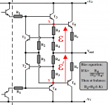
Folks, working from MH's equations given in the figure below, the following may be deduced:
1. Select R3 and R4 to bias the output stage, and
2. Establish the ratio R2/R1=R3/(R3+R4) for maximal error cancellation.
It is my understanding from this equation, and from the schematic below, that the error ''E'' is extracted from the output stage with respect to its input ''X'' and simultaneously attenuated according to the transfer function R3/(R3+R4).
Thus, transistor T1 receives E.R3/(R3+R4) at its base, and must thereafter amplify the signal by (R3+R4)/R3 to reverse the attenuation occasioned by voltage divider R3, R4.
It follows, therefore, that since T1's gain (in ''common-emitter'' mode) is approximately R1/R2, then, in order to restore unity-gain-transfer of error ''E'' through T1, gain provided by the later must be R1/R2=(R3+R4)/R3, which is identical to Hawksford result in (2) above.
Simultaneously, transistor T1 necessarily provides the inversion mandated by stylized summer S2 here.
Clearly, the above analysis also applies to the negative polarity, whose electrical point of reference is ''Y''.
From my perspective, therefore, this analysis demonstrates that, at balance, there is NO such thing as infinite feedback in this loop, and that my objections were entirely valid in fact. 😎
Now, Brain, if you have VALID objections to the above, arm yourself with cohesive and coherent evidence in rebuttal.

Attachment replaced per Mike's request -Mod team Dec, 04, 2006
Folks, working from MH's equations given in the figure below, the following may be deduced:
1. Select R3 and R4 to bias the output stage, and
2. Establish the ratio R2/R1=R3/(R3+R4) for maximal error cancellation.
It is my understanding from this equation, and from the schematic below, that the error ''E'' is extracted from the output stage with respect to its input ''X'' and simultaneously attenuated according to the transfer function R3/(R3+R4).
Thus, transistor T1 receives E.R3/(R3+R4) at its base, and must thereafter amplify the signal by (R3+R4)/R3 to reverse the attenuation occasioned by voltage divider R3, R4.
It follows, therefore, that since T1's gain (in ''common-emitter'' mode) is approximately R1/R2, then, in order to restore unity-gain-transfer of error ''E'' through T1, gain provided by the later must be R1/R2=(R3+R4)/R3, which is identical to Hawksford result in (2) above.
Simultaneously, transistor T1 necessarily provides the inversion mandated by stylized summer S2 here.
Clearly, the above analysis also applies to the negative polarity, whose electrical point of reference is ''Y''.
From my perspective, therefore, this analysis demonstrates that, at balance, there is NO such thing as infinite feedback in this loop, and that my objections were entirely valid in fact. 😎
Now, Brain, if you have VALID objections to the above, arm yourself with cohesive and coherent evidence in rebuttal.
Attachment replaced per Mike's request -Mod team Dec, 04, 2006
Attachments
Mike, go directly back to post #774, do not pass GO, do not collect $200. And read all the posts carefully from there until here before you waste any more disk space and time. This isn't a competition!
Re: Turkeys hide!
Post 774:
Incorrect!
Start again, self-evidently, from here!
Post 774:
traderbam said:Happy Thanksgiving to those who celebrate it!
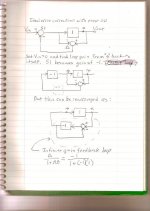
Now to calculate the gain of the feedback loop. Fig 8. is the simplified output stage (with the phases of G1 and G2 put right!) with the FETs removed (optional). The input is grounded and a voltage signal V1 is applied to the output. The ratio of v(n1) to V(out) or v(n2) to v(out) shows the gain of the loop.
I'll do the algebra in case anyone is interested.
The maths is tedious unless you assume perfect symmetry of the top and bottom halves. So assume gm1=gm2 and therefore v(n1)=v(n2). Remember, this is an ac analysis so dc levels are ignored.
The bottom half can now be ignored and effectively removed from the circuit.
Let i be the current through G1 and gm be the transconductance of G1.
v(fb0) = i.R4 + v(n1)
v(n1) = -i.R1
i = gm.[ v(fb1) - v(fb0) ] = gm.[ (v(n1) + v(out))/2 - i.R4 - v(n1) ]
substitute -v(n1)/R1 for i
-v(n1)/R1 = gm.v(n1)/2 + gm.v(out)/2 + gm.v(n1).R4/R1 - gm.v(n1)
which simplifies to
-v(out)/v(n1) = { 2.( 1 + gm.R4 )/(gm.R1) - 1 }
v(n1)/v(out) = - { (gm.R1) / [ 2 + gm.(2.R4 - R1) ] }
If you put in the values shown in the diagram, gm = 0.04, R1 = 680, R4 = 330, the ratio v(n1)/v(out) = -23.
The loop gain or "correction power" is 27dB. The real circuit will be different because the circuit values are different and there are some extra parts. Perhaps Andy or jcx would measure this in the full circuit simulation.
Incorrect!
Start again, self-evidently, from here!
Thanks jcx,
your scans from Horowitz in post 1116 seems to answer my previous question, whether the Hawksford error correction topology appears elsewhere in the literature. It seems clear that it is identical to fig. 6.1-1f. I suppose even you earlier reference to Åström might have answered my question too, but it wasn't as clear there.
I also think the excerpt from Horowitz makes things clearer (at least to me). I don't claim to say anything really new here, but I think Horowitz can help us to get a new view of the matter. If we look at fig. 6.1-1a (which is claimed equivalent to f) it looks like an ordinary feedback system, with the exception that an extra block is added at the plant input. Since it is a linear system (and if I am not mistaken) this block, just like all other transfer functions are of the form k*P(s)/Q(s) for some polynomials P and Q. That is, in fig a, we add a gain block (or less likely an attenaution block) possibly with compensation circuitry.
What distinguishes case a, which is a 2nd degree of freedom (DoF) system, from an ordinary feedback system, that is a 1st DoF system, is this extra gain block which we prepend to the plant. From the first paragraph of Horowitz' text we learn that when a 1st DoF system does not have sufficient loop gain to attain both design goals (the desired output and supression of disturbances), a 2nd DoF system may be considered to overcome this problem. Case a in the figure is then clear, since we can view it as a 1st DoF system turned into a 2nd DoF system by adding gain to the plant. That is, we increase the amount of OLG so we can achieve our design goals by ordinary feedback. Case f then, which is the Hawksford EC, is equivalent, but achieves the same purpose by attempting not to waste any OLG on feeding back the desired signal, but only feed back the undesired signal. One might perhaps say that it tries to use the available loop gain more cleverly instead of cranking it up to make ordinary feedback work.
A final observation would be that while control theory typically deals with adding control to a given plant, in audio we often design the plant itself simultaneously to designing the control system. Hence, adding Hawksford EC to a whole amplifier would be essentially equivalent to modifying the amp itself to have a higher OLG so that ordinary feedback is sufficient. Since we are designing the actual plant itself, there is no need to distinguish between the plant and the added gain block, as in case a. However, if we are working with a single stage or similar as our plant, we may not consider it an option to increase the OLG, in which case other topologies from Horowitz may be necessary.
Also please note that I do not try to imply that it does not matter in practice, on the circuit level, which topology we use in cases where they are equivalent. A certain topology may, for instance, be much simpler to implement so that it meets the desired design goals.
mikeks said:Christer, read the abstract in this patent, previously discussed in this post.
The Pichal patent? Yes, I had a brief look at it and I thought we had agreed it is basically equivalent to Hawksford EC, except that the amp is inverting. But I suppose it is dangerous to make assumptions about people agrreing in this thread. 🙂
What was your point?
Hi Christer,
Yes it does look, in principal at least, like the very idea written about by MH.
That was the point.

Seriously, Christer, have you found anything wrong with this position?
Cheers.
Yes it does look, in principal at least, like the very idea written about by MH.
That was the point.
Christer said:.....I suppose it is dangerous to make assumptions about people agreeing in this thread. 🙂
Seriously, Christer, have you found anything wrong with this position?
Cheers.
Christer said:[horowitz]What distinguishes case a, which is a 2nd degree of freedom (DoF) system, from an ordinary feedback system, that is a 1st DoF system, is this extra gain block which we prepend to the plant. From the first paragraph of Horowitz' text we learn that when a 1st DoF system does not have sufficient loop gain to attain both design goals (the desired output and supression of disturbances), a 2nd DoF system may be considered to overcome this problem. Case a in the figure is then clear, since we can view it as a 1st DoF system turned into a 2nd DoF system by adding gain to the plant. That is, we increase the amount of OLG so we can achieve our design goals by ordinary feedback. Case f then, which is the Hawksford EC, is equivalent, but achieves the same purpose by attempting not to waste any OLG on feeding back the desired signal, but only feed back the undesired signal. One might perhaps say that it tries to use the available loop gain more cleverly instead of cranking it up to make ordinary feedback work.
[snip]
Christer,
I fully agree with the last part of this. My only question would be: if H.ec indeed avoids cranking up OLG by only feeding back the error (and I believe this is the crux of the matter), does it than still satisfy the definition of 2DoF quoted above?
Jan Didden.
From andy_c's scan: ""Set Vin=0"
I assume you are doing this without loss of generality, for example only?
I assume you are doing this without loss of generality, for example only?
janneman said:
I fully agree with the last part of this. My only question would be: if H.ec indeed avoids cranking up OLG by only feeding back the error (and I believe this is the crux of the matter), does it than still satisfy the definition of 2DoF quoted above?
Jan,
I am no expert in control theory, but I think it is clear from the excerpts from Horowitz that this is the case. Case f in the figure seems to me to nail down the error correction suggested by Hawksford and Pichal, and all cases in the figure are claimed to be equivalent 2DoF systems. Note that the text does not require that we add gain to a 1DoF system to get a 2DoF system. It just states that we need to go to a 2DoF system if there is not enough OLG to solve our problem with a 1DoF system. As the various cases in the figure show, there are many ways to solve this problem. One of these ways, case a, is to add gain to the plant. Another way, case f, is to feed back only the error, which (without trying to calculate anything) I think lets us waste away all of the OLG on correcting the error, since we don't attenaute the input signal by feeding back any part of the desired signal (expressed a bit sloppy, but I think you get it). Note though, that just like jcx, I rely on what Horowitz writes and I haven't tried to check his claims (which I think can be safely considered as unnecessary).
mikeks said:
Yes it does look, in principal at least, like the very idea written about by MH.
That was the point.
OK, so your point was that the Pichal and Hawksford approaches are essentially equivalent, so, judging by patent dates, Pichal was much earlier than Hawksford to suggest applying Horowitz' case f to audio amplifiers? Yes, I would agree on that.
Patent engineers would probably say they are two different ideas, though. 🙂
I have honestly tried to avoid digging too deep into the details of many posts as long as people are disagreeing so vividly. But maybe it is futile to wait for some convergence first.? 🙂
I think I can agree to your equations in that post, although you make some assumptions I would have to think more about whether I can accept or not. I don't think it would make any fundamental difference, though, if I choose to disagree with some assumption.
If you are rather talking about the issue of positive feedback (assuming that is what you mean by infinite feedback), then I stand by what I said earlier, that it is possible to view the circuit as having two feedback loops, one positive and one negative, which are combined by superposition. Note however, the crucial distinction that somebody (I have forgotten who) made between feedback path and feedback signal. That is, if we choose to view the system as having two feedback paths (or loops), which is only one of several possible ways to view it, the actual signal being fed back is the result of superposition of both these paths. Hence, the existence of a positive feedback path does not necessarily imply the existence of positive feedback of the resulting feedback signal when more feedback paths are present. Further note, that this is only one of several equivalent possible ways to view the system. Whether one prefers to analyse it in this way or that way is a matter of preference.
Interestingly, however, I think block diagram operations Brian showed earlier, of isolating the positive feedback loop inside the negative one, and replacing it by a corresponding gain block actually shows how to convert from Horowitz' case f to case a. So for that particular purpose, it seems to have some merit to use the two-loop view.
Nixie said:From andy_c's scan: ""Set Vin=0"
I assume you are doing this without loss of generality, for example only?
For a loop gain calculation, the external input is set to zero, and a signal is injected inside the loop (at "x" in my diagram above) to measure the gain all the way around the loop back to where the signal was injected.
So in the standard feedback system with forward gain "A" and feedback factor "B", the loop gain is A*B. But to get that you have to set the external input to zero.
andy_c said:
Bob is right, Mike. See the loop gain calculation in the attachment.
Hi Andy, your analysis is incorrect.
This may be established by setting all the ''K'' terms here to unity.
This gives a loop gain of zero for zero error extracted; i.e. an ideal voltage follower.
- Home
- Amplifiers
- Solid State
- Bob Cordell Interview: Error Correction