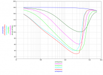
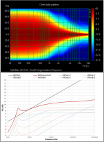
The following graphs result from running the segments each as second order rc-filter with segment voltage gain set to 0.1 at the frequency where lambda/2 is the panel diameter. This improves directivity. Whether those curves are viable regarding sensitivity, tweeter excursion capability and phase behavior I'm not able to model yet... At 180hz the outer panel is already down to a quarter of the input voltage for example; so the tweeter would do four times the excursion...
Attachments


The directivity patterns were generated using an Excel spreadsheet calculation of the generalized Walker Equation. I use a VBA macro to step thru different angles and output impulse response files that can be read into ARTA for plotting directivity. If you are not familiar with the Walker Equation and/or ESL operation, you might find this document useful. http://home.kpn.nl/verwa255/esl/ESL_English_2011.pdf… May I ask, how did you generate that directivity pattern? (expert software, analytical insight?)
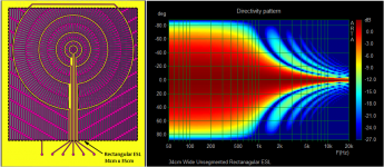
Attached is horizontal directivity pattern for your 34cm wide rectangular panel if it was driven uniformly.Could you make a directivity pattern of a simple rectangular panel of same proportion for comparison?
The easiest way, is to use a resistive ladder network(ie RC transmission line). As you work outward in segments, you retain the roll-off from the previous segment and add an additional 1st order slope. I’ll post an example shortly.… I can't think of an easy way to steepen the low-pass passively after the transformer.
Attachments
The following graphs result from running the segments each as second order rc-filter with segment voltage gain set to 0.1 at the frequency where lambda/2 is the panel diameter. This improves directivity. Whether those curves are viable regarding sensitivity, tweeter excursion capability and phase behavior I'm not able to model yet... At 180hz the outer panel is already down to a quarter of the input voltage for example; so the tweeter would do four times the excursion...
The Walker Equation for ESLs can relate pressure in the far field to panel dimensions and applied voltages:
P = e0 * Vsig * Vpol * A * f / (2 * d^2 * c * r)
Where:
P = sound pressure (N/m^2)
Vsig = signal voltage applied to stators
Vpol = bias voltage applied to diaphragm
A = area of ESL (m^2)
f = frequency (hz)
d = stator to diaphragm spacing (m)
c = speed of sound (m/s)
r = listening distance (m)
e0= electric constant
Note that:
- with constant stator voltage, far field pressure is proportional to frequency (ie increases +6dB/oct)
- there is a limit to the voltage that can be applied before the air in the gap will ionize and conduct and/or arc. This puts a ceiling on the max SPL that can be generated for a given panel area. Increasing the gap size does not increase the max SPL, it just increased the voltages required to achieve that SPL. If interested, more details can be found in the Baxandal ESL chapter.
P. J. Baxandall, “Electrostatic Loudspeakers,” in
Loudspeaker and Headphone Handbook, J. Borwick, Ed.
(Reed Educational and Professional Pub., Woburn, MA,
1998), pp. 106–195.
Also here is a link showing what happens when you exceed the ionization voltage gradient in the gap,
and a link on how to set optimum bias voltage.
First time ESL builder
Measured my ESL attempt
Attachment #1 Directivity Plot and individual segment contributions to SPL @ 1m on-axis for the filtering shown in Post #5
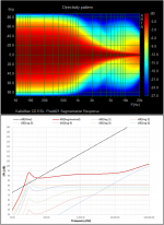
Attachment #2 Directivity Plot and individual segment contributions to SPL @ 1m on-axis for the filtering shown in Post #21
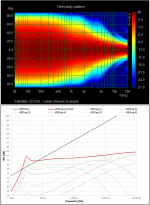
Attachment #3 Directivity Plot and individual segment contributions to SPL @ 1m on-axis for an example ladder resistor network. This is by no means optimized, but you can see that usefully broad polar can be achieved. In this case, I actually combined the inner 2 segments since the output from the first segment was so small on it’s own there wasn’t any benefit to separating it.
*** In attached plots, an estimate of the max possible SPL @ 1m on-axis for unsegmented panel is shown as a dashed black line.
Also note that I set a notional diaphragm resonance of 30Hz with Q=4
Attachments
Last edited:
Acoustic lens like the on the russian guy used. That is a clever way to increas the area and by that the sensitivity without risking an arc.
Or buy yourself a set of QUAD esl63s and you are done! 🙂
Or buy yourself a set of QUAD esl63s and you are done! 🙂
I also have beveridge 2sw2 speakers.
Sounds totally amazing after som EQing.
Beveridge relies on its lens, thats what makes that speaker so unique and wonderful.
Sounds totally amazing after som EQing.
Beveridge relies on its lens, thats what makes that speaker so unique and wonderful.
So you have receipe for good esl - stack 3xESL57 bass panels vertically and use small tweeter panel with lens in the middle with adjustable angle.


- Home
- Loudspeakers
- Planars & Exotics
- An attempt at a constant dipolar directivity esl panel