Interesting new feature at https://amcoustics.com/tools/amroc-pro , non shoebox room models:

Here a floorplan of my groundfloor.
Seems to correlate reasonably well with measured room modes.
Here a floorplan of my groundfloor.
Seems to correlate reasonably well with measured room modes.

I have been intermittendly working on my speakers, working with Acourate is now becoming proficient.
At the moment i am playing with target curves at the main listening position (MLP) to get a feeling for the effect on enjoyment of music.
Just a note: i was also compensating the spl loss, but that created very funny distortions, like drivers were rattling at high pitch of sorts with the midrange and/or tweeter, and the woofer sounding i do not know how to word it, but not good ;-).
So i did not do any compensation and immedeately those funny distortions were gone, so redid all target curved filters.
To give a peak into this, here some target curves based on looking at target curves that appear to be working well for the person publishing it:

Note: normalised at 714Hz, just to show the balance differences, and T5 being with the tick line, being the curve that at first evaluation i liked best.
I am still amazed how different the balance of those tartets is, cannot get my head around, but i went ahead and found T5 to be for me the better one, perhaps a fraction hot on certain albums, but on known good recordings was already very good. Also my wife noticed the differences, and actually played with the volume a bit, for me a sign it is very good already.
Based on T5 i made T6 with a bit stronger drop in higher frequency, this one is perhaps more forgiving.
Here the differences:

The thick line is T6, so appears to be not much difference, but for the listening it does. By the way the red curve is the response without the driver level corrections and corrections for the room influences. And shows the first room modes quite well. Check the post on the room simulation, it has a decent correlation.
Note:

The target curves for T5 and T6, and the differences are not large, yet the subjective effect on the music is apparent, so interesting area to deepen my understanding. One aspect being the perceived equal loudness ;-) :


As a final not for this post, i have no clue as how my hearing determines how loud music sounds other than it is the midrange if there is no uncorrelated distortion (sounds) present. Or perceives those balance differences. All in all great fun in current state of the development.
At the moment i am playing with target curves at the main listening position (MLP) to get a feeling for the effect on enjoyment of music.
Just a note: i was also compensating the spl loss, but that created very funny distortions, like drivers were rattling at high pitch of sorts with the midrange and/or tweeter, and the woofer sounding i do not know how to word it, but not good ;-).
So i did not do any compensation and immedeately those funny distortions were gone, so redid all target curved filters.
To give a peak into this, here some target curves based on looking at target curves that appear to be working well for the person publishing it:
Note: normalised at 714Hz, just to show the balance differences, and T5 being with the tick line, being the curve that at first evaluation i liked best.
I am still amazed how different the balance of those tartets is, cannot get my head around, but i went ahead and found T5 to be for me the better one, perhaps a fraction hot on certain albums, but on known good recordings was already very good. Also my wife noticed the differences, and actually played with the volume a bit, for me a sign it is very good already.
Based on T5 i made T6 with a bit stronger drop in higher frequency, this one is perhaps more forgiving.
Here the differences:
The thick line is T6, so appears to be not much difference, but for the listening it does. By the way the red curve is the response without the driver level corrections and corrections for the room influences. And shows the first room modes quite well. Check the post on the room simulation, it has a decent correlation.
Note:
- The pulse response and the phase response show there is a minimal timing difference between drivers , probably tweeter being a fraction late. It is within 1 perhaps 2 samples though (sampling frequency/rate : 48K/65536).
- The curves are smoothed using Acourate's macro1 doing a psycho-acoustic smoothing, using the standard settings, with the result being minimum phase.
- All filters have a 20Hz high-pass applied when creating the filter:
The target curves for T5 and T6, and the differences are not large, yet the subjective effect on the music is apparent, so interesting area to deepen my understanding. One aspect being the perceived equal loudness ;-) :
As a final not for this post, i have no clue as how my hearing determines how loud music sounds other than it is the midrange if there is no uncorrelated distortion (sounds) present. Or perceives those balance differences. All in all great fun in current state of the development.
Going back to the publications of room curves, Toole et al, the controverse is whether it is a result or a target. Toole states clearly it is a result, B&K i am not so sure, also the appreciation by listeners varies a lot.
In my case, creating an more or less anechoic on-axis and off-axis response is not possible due to physical problems after a car accident. Given the above i am not so sure that it will help me a lot.
So instead i used my on/off axis measurements at 100cm from baffle of Mindrange and Tweeter to make a "dead reckoning" ;-) of the estimated inroom curve. Then use this to define a target curve at listening position rel to mid/tweeter (3068mm).

From these curves it is clear that the off-axis response has a smooth behaviour(the Akabak sims do work ;-)), and the differences between on-axis and est inroom coincide more or less at crossover M-to-T. So useable to get values to use in Acourate to create a target:

The issue is still the range below 433Hz , this curve is latest of a few , with previous curves the range between ~ 100 and 500 Hz has a very noticable effect on voices in particular, and for me it appears to be an area also for the mixing/mastering to play given the differences between recordings. So boils down to personal preferences ;-)
Same for the high end, where for me the effect on the perceived distance of the voice/instrument, again a area where it will be a balance between preference and overall effect on the perceived dynamics.
In my case, creating an more or less anechoic on-axis and off-axis response is not possible due to physical problems after a car accident. Given the above i am not so sure that it will help me a lot.
So instead i used my on/off axis measurements at 100cm from baffle of Mindrange and Tweeter to make a "dead reckoning" ;-) of the estimated inroom curve. Then use this to define a target curve at listening position rel to mid/tweeter (3068mm).
From these curves it is clear that the off-axis response has a smooth behaviour(the Akabak sims do work ;-)), and the differences between on-axis and est inroom coincide more or less at crossover M-to-T. So useable to get values to use in Acourate to create a target:
The issue is still the range below 433Hz , this curve is latest of a few , with previous curves the range between ~ 100 and 500 Hz has a very noticable effect on voices in particular, and for me it appears to be an area also for the mixing/mastering to play given the differences between recordings. So boils down to personal preferences ;-)
Same for the high end, where for me the effect on the perceived distance of the voice/instrument, again a area where it will be a balance between preference and overall effect on the perceived dynamics.
Just regular listening to filters with different targetcurves for some time then switch, it seems we (my wife and i) prefer the curve that is based on the directivity synthesis in previous post, but with lower frequencies less pronounced. Actually it is sort of equal to the B&K curve. Perhaps a bit less drop above 10kHz will be the next update. Also a time align is performed some 20 samples (65536) of Bass vs Tweeter (and mid 1 sample), but not sure about bass, as measurement also contains room modes. If i neglect room modes it is 2-4 samples. I sounds slightly different, but to contain cognitive bias i will switch between the two latest at intervals of 2-3 days.
Before time align:

After time align:

Note: some small differences due to a small increase in toe-in, thus also mic position. Aslo in both cases a highpass filter at 20 Hz.
I noticed small SPL level difference between shape-wise identical target curves. Will redo this to eliminate possible effects. Anyhow, given the corrected filters for bass and mid it is clear that around the 433Hz crossover some differences are apparent. How audible these differences are remains to be heard ;-)
Enyoing music, that is for sure. Also the sound space of the music sort of blends seamlessly with the soundspace of our living room soundwise. When music stops it is not as if i switch to another sound space. Very nice.
Before time align:
After time align:
Note: some small differences due to a small increase in toe-in, thus also mic position. Aslo in both cases a highpass filter at 20 Hz.
I noticed small SPL level difference between shape-wise identical target curves. Will redo this to eliminate possible effects. Anyhow, given the corrected filters for bass and mid it is clear that around the 433Hz crossover some differences are apparent. How audible these differences are remains to be heard ;-)
Enyoing music, that is for sure. Also the sound space of the music sort of blends seamlessly with the soundspace of our living room soundwise. When music stops it is not as if i switch to another sound space. Very nice.
An update on my "Alice in Wonderland " journey. Focus on targetcurve.
Some hindering due to health issues over here, but first of all the current active filter version (V17) allows us to enjoy music.
The number 'hides' the total number of filter versions, times 3 is more appropriate.
The objective is not to learn the basic tool, that was already achieved, but the audibe and measurable effect of the choices to make during creation of a filter.
The first choice i settled on , at least for now, is the target curve. So i scanned the internet and here just a set of what i found:
As all of there were also described audibly, i find it very remarkable of they differ!
And yes i tried some of them, and found them sound remarkably different.
So back to the drawing board, and first of all studied o-Toole's / Sean Olive's publications on house curves, basically their principle: the room curve is an outcome of the radiation behaviour of the loudspeakers, and not a Target perse!
Smooth and straight online and offline spl curves (in anechoic condition) is the core requirement. But i do not have the capability to measure in anechoic conditions, so measurements are done in my living room at 100cm from baffle, just the midrange an the tweeter in steps of 10 degrees horizontal. With the SPL curves loaded in Vituixcad i could get a indication of in room response and directivity.
THis outcome sort of matched the B&K curve , of which i found a set of spl points on aktiveshoere.de, so loaded as spl curve in Acourate and adjusted to make it smooth and to match the assumed behvious shown in VituixCAD. I also tried to replicate this in Macro 2 (creation of target curve) but somehow could not get it close enough. So i used the manually constructed curve (target11a) as target.
Here a screencopy :
THis curve Target11a is in use now for a month or so, and we are happy with it, except for some concern in the low bass region.
So the next focus is the bass performance, and the first aspect is the rumble filter in Macro 4 (filter files creation) , so i use 20, 15, 10 Hz and alternatevely listen to one or the other.
This image also shows the issues in the bass region. The group delay curves are of interest as well as the peaks seem to align with the peaks in the spl.
So i am studying options to mitigate these, given that the basic speaker placement in my living room is a given, as is the arrangement of the room so no bass traps etc.
Note: to smoothen the spl curves is use acourate Macro1 which does an approximation of how we "hear" the spl curves.
Nice!
@JanRSmit: I assume you run the woofers with one channel (parallel or series). Have you tried adding inductor in series with lower woofer?
I have seen that @mayhem13 have pointed that tip in some other threads.
I have tried with two drivers having about same distance as in my next build. Then feed them with a channel of DSP each. Lower woofer get additional 6dB filter at 1000 hz (DSP). I have tried with filter at 200 Hz LR12 and no filter.
With 6 db on lower woofer "simulate inductor": sound is darker and more tight. Play more like one driver than two with some distance.
No 6 dB: Sound is brighter more all over the place. A bit like to many artist playing lead at the same time.
Inductor in good in good quality is not cheap....At least the testing with DSP is free 🙂
It is on my list of options to test.
My woofers are connected in parallel to a amplifier channel. So i consider a inductor , i have a few of very good quality😎
Will seek the posts of @mayhem13
My woofers are connected in parallel to a amplifier channel. So i consider a inductor , i have a few of very good quality😎
Will seek the posts of @mayhem13
Looking forward to hear about that test!
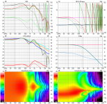
I tried simulating was is going on in VituixCAD when inductor is added to lower woofer.
Of course this is not something new, but more often that not, 3 way today is with only one woofer.
Im not a connaisseur in Vituix CAD, but here is my take. True or not:
Open diffraction tool and simulate two 8" woofers. Checkmark directivity then export.

Make new project in VituixCad. Add simulated measurements to drivers.
Take shortcut and pick 3 way active block from library
Baseline one driver only. No filter applied:


Adding second woofer with no filter:


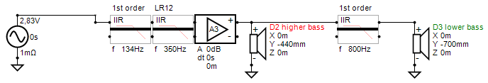
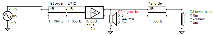
Adding inductor / 1st order filter at 800 hz

Adding LR12 at 350 hz without "inductor


Finally Adding "inductor" to lower woofer and also LR12 at 350 hz.


I tried simulating was is going on in VituixCAD when inductor is added to lower woofer.
Of course this is not something new, but more often that not, 3 way today is with only one woofer.
Im not a connaisseur in Vituix CAD, but here is my take. True or not:
Open diffraction tool and simulate two 8" woofers. Checkmark directivity then export.
Make new project in VituixCad. Add simulated measurements to drivers.
Take shortcut and pick 3 way active block from library
Baseline one driver only. No filter applied:
Adding second woofer with no filter:
Adding inductor / 1st order filter at 800 hz
Adding LR12 at 350 hz without "inductor
Finally Adding "inductor" to lower woofer and also LR12 at 350 hz.
Attachments

Last edited:
I am now not in my workshop, but will show with vituixcad what i have as an option tobtest. Requires a 3,9 mH inductir for the lower woofer.
For the active filtering i use Acourate, not an option jn Vituixcad.
For the active filtering i use Acourate, not an option jn Vituixcad.
As promised @Rokytheman , here the option on my list of options to test ;-)
It shows the on and off axis response at 100cm on-axis measurements at the real positions in space, with near-field(5mm) merging for the bass response.
In my case it requires a 3.9mH inductor (0.18Ohm) which i happen to have:

Effectively i loose little if any SPL.
It shows the on and off axis response at 100cm on-axis measurements at the real positions in space, with near-field(5mm) merging for the bass response.
In my case it requires a 3.9mH inductor (0.18Ohm) which i happen to have:
Effectively i loose little if any SPL.
Also for the tweeter it is on the list of options to test, depens on when the purifi tweeter will arrive 🙄
This is a measurement at 100cm on -off axis.

And to get rid of the breakup at 25kH, as an option as well:

This is a measurement at 100cm on -off axis.
And to get rid of the breakup at 25kH, as an option as well:
Last but not least, also for the midrange, with its breakup peak at ~8.3kH:


For reference, the cross-over frequencies are 433 and 3464Hz, a special version from Acourate, effectivly not wider than 1 octave below/above Fr, but starts relatively soft, at Fc it is -6dB. So 216-866Hz and 1732-6928Hz)
For the midrange it means that the cone breakup is outside of the passband, nevertheless , it can be of benefit.
But first the focus is on the room influence in the lower bass region ;-)
Purifi 8" vs SS21W, Of course from memory, but clarity or transparent, can play a lot louder without loosing quality.
Purifi has begun delivery of their tweeter, the 104mm version. So i did some digging in results of last year major upgrade and raw measurements of drivers in the enclosure to show that the 104mm tweeter (SB26ADC with 4" oval waveguide) could match quite well with a 4" PTT4.0M08-NAC04.
Here the Predicted In-Room-Curves as created in VituixCAD based on horizontal 10 degree step off-axis measurements 0-180 degrees:

The violet curve is the SB26ADC with a 4" oval waveguide (based on the 4" version of @augerpro ), the mint-blue is the PTT4.0M08-NAC4 . The XO Fs is 3464Hz, and acts in 2 octaves, so pretty steep (see the 3 markers). The shape of the baffle for midrange and tweeter are optimized with simulation with Akabak for a smooth off-axis response and wide as possible transition zone for the midrange.
To summarise, i hope the Purifi tweeter will give a similar "fit" at the XO range, be it with probably a more flat(horizontal) in-room response in the range above the XO. Fingers crossed 😎
Here the Predicted In-Room-Curves as created in VituixCAD based on horizontal 10 degree step off-axis measurements 0-180 degrees:
The violet curve is the SB26ADC with a 4" oval waveguide (based on the 4" version of @augerpro ), the mint-blue is the PTT4.0M08-NAC4 . The XO Fs is 3464Hz, and acts in 2 octaves, so pretty steep (see the 3 markers). The shape of the baffle for midrange and tweeter are optimized with simulation with Akabak for a smooth off-axis response and wide as possible transition zone for the midrange.
To summarise, i hope the Purifi tweeter will give a similar "fit" at the XO range, be it with probably a more flat(horizontal) in-room response in the range above the XO. Fingers crossed 😎
Privately we are going through some difficult times, as some people close to us passed away. But as a sort of distraction i measured again the effect of a parallel RLC in series with the PTT4.0M08-NAC04 midrange to surpress its 8.3kHz cone breakup peak. I have done it several times just to be sure measurement variations are not in play.
The SPL without and with RLC:

To eliminate effects of SPL differences, i created a spl-phase-linear filter using the same target passband 433-3464Hz(shown in pictures as grey zone), and measured distortion of both. The software used is Acourate. Shown is the spl measured (K1), and the K3 and K5 of without and with RLC in place, Voltage is 2,84Vrms, distance 315mm from baffle, mic is a calibrated Beyerdynamic MM1:
The K1 curves overlap near perfectly. The K3 and K5 curves are shown at the K1 frequncy where the K3 and K5 occur .
K3 of NoRLC highlighted (brown curve) vs K3 of YesRLC(Blue curve):


So significant difference in K3 measured. Also in K5 some difference but less pronounced.
So i listened also to this set-up, so nly the midrange filtered, in both setup's requiring not only swapping the RLC filter in-out, but also the created filters.
So it is more memory than instant A-B switching, but on voices (pop, classic (Bach requiem) i would say the RLC filter makes the pronounciation (consonnant attack) better. A certain sharpness is gone, making the tone more coherent, yet as dynamic. Do not know if my wording gets the impression across.
My conclusion: Worthwhile to add to my GAYA2-Purified system. And also for the conebreakup peak of tweeter.
As a closing note:
The reason creating a ampl-phase linear passband for both cases is also that i wanted to eliminate also the impact of phase(time) differences introduced by the RLC.
The SPL without and with RLC:
To eliminate effects of SPL differences, i created a spl-phase-linear filter using the same target passband 433-3464Hz(shown in pictures as grey zone), and measured distortion of both. The software used is Acourate. Shown is the spl measured (K1), and the K3 and K5 of without and with RLC in place, Voltage is 2,84Vrms, distance 315mm from baffle, mic is a calibrated Beyerdynamic MM1:
The K1 curves overlap near perfectly. The K3 and K5 curves are shown at the K1 frequncy where the K3 and K5 occur .
K3 of NoRLC highlighted (brown curve) vs K3 of YesRLC(Blue curve):
So significant difference in K3 measured. Also in K5 some difference but less pronounced.
So i listened also to this set-up, so nly the midrange filtered, in both setup's requiring not only swapping the RLC filter in-out, but also the created filters.
So it is more memory than instant A-B switching, but on voices (pop, classic (Bach requiem) i would say the RLC filter makes the pronounciation (consonnant attack) better. A certain sharpness is gone, making the tone more coherent, yet as dynamic. Do not know if my wording gets the impression across.
My conclusion: Worthwhile to add to my GAYA2-Purified system. And also for the conebreakup peak of tweeter.
As a closing note:
The reason creating a ampl-phase linear passband for both cases is also that i wanted to eliminate also the impact of phase(time) differences introduced by the RLC.
The PURIFI PTT1.3T04-HAG-01 arrived yesterday!

The start of the final seps to complete the Purification of my loudspeakers. So this is the last post in this thread, and i will open a new thread called:
GAYA2P The Purification completed
The start of the final seps to complete the Purification of my loudspeakers. So this is the last post in this thread, and i will open a new thread called:
GAYA2P The Purification completed
- Home
- Loudspeakers
- Multi-Way
- GAYA2-Final, finishing the unfinished after 15 years