You can run ARTA in demo mode, import *.wav files and generate Burst decays if you want.Burst decay was mentioned to me by a fellow person on facebook. but i dont have arta 🙁
I'm not sure why that would be.People also mentioned you need a mic that can at least go much higher in frequency (min does 20khz) response to be able to measure this correct.. it sound weird to me is that true ?
Thanks for the *.wav file. I should have some time tomorrow to put together a few different plot trends to help explain what the different CSD settings do and how best to use them. Will also try to explain the pros and cons of CSD vs Burst vs Spectrogram.i measured at around 25 cm or something. to get the background noise down.
Any chance of getting a near-field measurement at 1cm from the center of the ribbon? That should help to understand what may or may not be happening in the 500Hz - 1500Hz range.
Are you saying that if you have a ceramic magnet and a neo magnet of exactly the same size and shape, ignoring the actual field strength, the flux distribution/shape/uniformity is different?ceramics have a better "reach out" than neos
size for size you get a more uniform field strength with ceramics
Thanks for your input on waterfall Bolserst
yes. ceramics field are more "uniform" than neos
A few years back I was working on wider ribbons and doing a bunch of field uniformity testing with different magnet arraignments. At the time I had access to a hall sensor the size of a pin head mounted to precision XYZ stages, so I could easily map out the field strength/ uniformity.
The Neos are obviously much stronger than ceramics BUT that strength changes very non linearly as you get closer to the magnet. The ceramics do too of course but not as much as the neos.
Are you saying that if you have a ceramic magnet and a neo magnet of exactly the same size and shape, ignoring the actual field strength, the flux distribution/shape/uniformity is different?
yes. ceramics field are more "uniform" than neos
A few years back I was working on wider ribbons and doing a bunch of field uniformity testing with different magnet arraignments. At the time I had access to a hall sensor the size of a pin head mounted to precision XYZ stages, so I could easily map out the field strength/ uniformity.
The Neos are obviously much stronger than ceramics BUT that strength changes very non linearly as you get closer to the magnet. The ceramics do too of course but not as much as the neos.
"Any chance of getting a near-field measurement at 1cm from the center of the ribbon? That should help to understand what may or may not be happening in the 500Hz - 1500Hz range."
This has so far been the only reliable way for me to "see" whats going on down there. Close mic , low volume, and longer time window.
I also seem to have to get the mic very close ( about 1/4 ") and at 90 degrees to ribbon, to avoid reflections off magnet structures?? This is with a free swinging ribbon with magnets to the sides. Not sure the issue but can see strange things in the "energy storage" window if mic isnt close enough and somewhere in the literature that came with measurement system ( Omnimic) it talks about these reflections. This is not in the "waterfall" window but the "energy storage" window. Not sure the difference between the two
Last edited:
You can run ARTA in demo mode, import *.wav files and generate Burst decays if you want.
I'm not sure why that would be.
Thanks for the *.wav file. I should have some time tomorrow to put together a few different plot trends to help explain what the different CSD settings do and how best to use them. Will also try to explain the pros and cons of CSD vs Burst vs Spectrogram.
Any chance of getting a near-field measurement at 1cm from the center of the ribbon? That should help to understand what may or may not be happening in the 500Hz - 1500Hz range.
Thanks again ! about the arta thing thats a nice workaround 🙂 !i remember that depending on the pros and cons 😉 haha thx !
i wikll try making a really close up measurement ! if i can !
and thanks for all the effort !
Thanks for your input on waterfall Bolserst
yes. ceramics field are more "uniform" than neos
A few years back I was working on wider ribbons and doing a bunch of field uniformity testing with different magnet arraignments. At the time I had access to a hall sensor the size of a pin head mounted to precision XYZ stages, so I could easily map out the field strength/ uniformity.
The Neos are obviously much stronger than ceramics BUT that strength changes very non linearly as you get closer to the magnet. The ceramics do too of course but not as much as the neos.
lowmass thats so funny , im my video i talk about this, and saying thati believe the surface flux of a neo is much much higher then comparable ferite. as in the ratio. thats weird where did i pick that up. for all i know it might be a post of yours ? really have no clue. haha
Question ! i was tryin to measure this weird driver YouTube
i am no expert in taking measurements. so i compared some settings from cumulative spectral decay measurements from this video of new record day alias GR audio. since i want to to make those plots to and be able to help me in maybe changing stuff for the better.
here are the examples i used YouTube
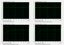
And made this measurement. and a picture of my settings , if you see something completely out of wack let me know.
Window used 4ms
CSD on
time window 4ms
rise time 0.6.
in the video they used 0.58ms not sure what that matters.
I adjusted the bottom floor to -25dB from the overall spl not the peak at 3Khz just as i see in the clio measurements from GR. although they do use the peak , then there would be less detail, i thought this might be more fair.
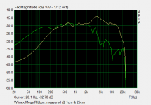
Ii measured at 0.25 meter and compensated the SPL for it. so the spl seen is actual spl at 1 meter. to get my room and noise floor down. (i know for such a huge thing also not ideal in frequency response to measure that close, but thats not what i am looking for now)
Driver tested is the big ribbon.
Looking at your CSDs starting at 300 Hz for the first trace, I guess you used an impulse response of about 3.3 ms length. That's what's typically possible as an anechoic measurement in a home environment. The next few traces use shorter and shorter pieces of the impulse response. As far as I can tell from your description, the last trace in the CSD would be 4 ms shorter than the first trace. That would be negative in your case... weird.
Here a 1 cm distance measurement. i must say i ddi change some horizontal alumnium strips to stiffen up the sides. since the sides tend to flap more since tjhey are not supported by the rest of the foil. also the lwoer first 4 cm is not corrugated 🙁 since after changin something i could only corrugate as far as my crimper would let me. since i did not make the whole thing interchangeable..... dumb next version i will be able to just remove the whole thing and try stuff.
Thanks for all the help !
Thanks for all the help !
Attachments
Looking at your CSDs starting at 300 Hz for the first trace, I guess you used an impulse response of about 3.3 ms length. That's what's typically possible as an anechoic measurement in a home environment. The next few traces use shorter and shorter pieces of the impulse response. As far as I can tell from your description, the last trace in the CSD would be 4 ms shorter than the first trace. That would be negative in your case... weird.
not even sure what you are saying here 🙂 (more my lack of knowledge when it comes to this then anything else) hihi. i used a window of 4ms int he measurement, and it is measured at 0.25 meter hope that helps ?
lowmass thats so funny , im my video i talk about this, and saying thati believe the surface flux of a neo is much much higher then comparable ferite. as in the ratio. thats weird where did i pick that up. for all i know it might be a post of yours ? really have no clue. haha
I have experienced many things over the years like you mention.
I see 2 possibilities...
1- Perhaps because of the intensity of their force you easily felt the effect of that non linearity when handling the neos , and from there concluded that they are more non linear than the ceramics.
OR
2- Your ability to discern the difference in their non linearity is finer than you expected.
I suspect #2 is quite possible because I often find that my brain is making connections/ keeping track of/comprehending things I am not directly consciously aware of.
I look forward to meeting its maker one day 😉
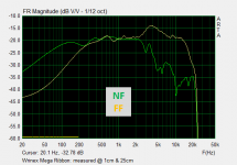
Thanks for the NF measurement 🙂Here a 1 cm distance measurement.
Comparing with the FF measurement really makes we wonder what is causing the 3-4kHz hump in the FF response. I thought perhaps baffle diffraction, but if the size is as 15cm x 20cm I don’t see how that is possible. You are running it as a dipole correct?
Attachments
My experience leads me to think the 3k hump may be bending mode of the rigid corrugated structure that is nulled out in FF.
I would move the mic around in front of diaphragm ( close mic )and see if that hump is gone in some areas of diaphragm (a null point)
you may need to get the mic really close to see it, like 10mm
I would move the mic around in front of diaphragm ( close mic )and see if that hump is gone in some areas of diaphragm (a null point)
you may need to get the mic really close to see it, like 10mm
Last edited:
... put together a few different plot trends to help explain what the different CSD settings do and how best to use them. Will also try to explain the pros and cons of CSD vs Burst vs Spectrogram
To compare and contrast the information displayed by CSD, Burst Decay, and Spectrogram plots I decided to create a set of 4 test signals.
Attachment #1:
1) Flat response with +3dB/Q=10 resonances at 500Hz and 5kHz
2) Same as 1) + first order HP filter @ 100Hz
3) Same as 1) + second order HP filter @ 100Hz
4) Same as 1) + reflection at 5mS and -20dB level
Attachment #2: Plot Comparison of signal 1)
CSD clearly shows the two resonances, but the 500Hz looks more severe because CSD has resolution that decreases with frequency. Also, since display axis is time, lower frequency resonance that decay in the same number of cycles as higher frequencies will look like they are worse as they hang on all across the plot. By comparison Burst Decay shows both resonances with equal resolution dying out at the same rate. The Spectrogram is a mix in that it shows both resonances at the same width(ie resolution) but since display axis is time, again the lower frequency resonance looks worse.
Attachment #3: Plot Comparison of signal 2)
Adding a simple first order HP filter 2 octaves below the resonance is pretty disruptive to the CSD plot making it look like there is another resonance involved. This is often the cause of the LF messiness of published CSDs. The Burst and Spectrogram plots look mostly unchanged as they should be.
Attachment #4: Plot Comparison of signal 3)
The second order HP filter is representative of the natural roll off of most transducers. Again, the CSD display could easily be misunderstood. Note in the Spectrogram the dashed line following the peak energy gives you a visual display of the group delay. This can be quite useful in more complex systems with crossovers.
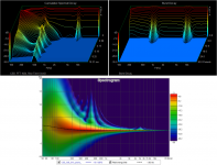
Attachment #5: Plot Comparison of signal 4)
Most measurements we take include some reflections. If not windowed out, they can add shelves or steps in the CSD plot depending on the length of the FFT window. Usually they have a rather mottled or boiling appearance. The Spectrogram will clearly show reflections as horizontal bars, as shown at the 5mS time axis. Reflections show up as curved traces on Burst Decay plots since signal is plotted in cycles not time.
Attachment #6: Alternate Burst Decay plot of signal 4), which often makes it easy to see you have a resonance AND a reflection happening.
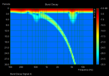
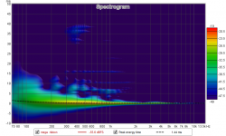
Attachment #7: Your 25cm Mega Ribbon measurement shows a few reflections arriving at roughly 6mS, 10mS and 16mS.
Let me know if you have any questions.
Next posting(tonight?) will go over each of the settings for the each plot type and show how they affect what is shown.
Attachments


Sorry, I should have labeled the plot curves. The 3K hump is in the FF, not in the NF.My experience leads me to think the 3k hump may be bending mode of the rigid corrugated structure that is nulled out in FF.
I agree about the possibility of NF measurements picking up local peaks from resonance modes in the diaphragm. Not sure if you had seen it, but I posted some plots and a short video showing model behavior using NF measurements along the length of an ESL pretty much all of which cancel out at the FF listening position. Another segmented ESL
Attachments
Last edited:
Great stuff thanks Bolserst
with the Omnimic system there is a window they call " energy storage". In this window I think I see "reflections" as you show in attach #5
In my limited understanding I have been using the waterfall window BUT I always switch to the energy storage window to see whats a reflection and what isnt.
Am I getting that right? At least in a limited way ha.
I will dig in deeper with your posts at some point but does above make any sense?
Actually looking again at your posts it looks like the spectrogram may be the easiest to "see" if something is a reflection?
Last edited:
Thanks for the NF measurement 🙂
Comparing with the FF measurement really makes we wonder what is causing the 3-4kHz hump in the FF response. I thought perhaps baffle diffraction, but if the size is as 15cm x 20cm I don’t see how that is possible. You are running it as a dipole correct?
Yes its running dipole. Further in the room the peak is less.
My experience leads me to think the 3k hump may be bending mode of the rigid corrugated structure that is nulled out in FF.
I would move the mic around in front of diaphragm ( close mic )and see if that hump is gone in some areas of diaphragm (a null point)
you may need to get the mic really close to see it, like 10mm
Ok ill try that this weekend !
To compare and contrast the information displayed by CSD, Burst Decay, and Spectrogram plots I decided to create a set of 4 test signals.
Attachment #1:
1) Flat response with +3dB/Q=10 resonances at 500Hz and 5kHz
2) Same as 1) + first order HP filter @ 100Hz
3) Same as 1) + second order HP filter @ 100Hz
4) Same as 1) + reflection at 5mS and -20dB level
Attachment #2: Plot Comparison of signal 1)
CSD clearly shows the two resonances, but the 500Hz looks more severe because CSD has resolution that decreases with frequency. Also, since display axis is time, lower frequency resonance that decay in the same number of cycles as higher frequencies will look like they are worse as they hang on all across the plot. By comparison Burst Decay shows both resonances with equal resolution dying out at the same rate. The Spectrogram is a mix in that it shows both resonances at the same width(ie resolution) but since display axis is time, again the lower frequency resonance looks worse.
Attachment #3: Plot Comparison of signal 2)
Adding a simple first order HP filter 2 octaves below the resonance is pretty disruptive to the CSD plot making it look like there is another resonance involved. This is often the cause of the LF messiness of published CSDs. The Burst and Spectrogram plots look mostly unchanged as they should be.
Attachment #4: Plot Comparison of signal 3)
The second order HP filter is representative of the natural roll off of most transducers. Again, the CSD display could easily be misunderstood. Note in the Spectrogram the dashed line following the peak energy gives you a visual display of the group delay. This can be quite useful in more complex systems with crossovers.
Attachment #5: Plot Comparison of signal 4)
Most measurements we take include some reflections. If not windowed out, they can add shelves or steps in the CSD plot depending on the length of the FFT window. Usually they have a rather mottled or boiling appearance. The Spectrogram will clearly show reflections as horizontal bars, as shown at the 5mS time axis. Reflections show up as curved traces on Burst Decay plots since signal is plotted in cycles not time.
Attachment #6: Alternate Burst Decay plot of signal 4), which often makes it easy to see you have a resonance AND a reflection happening.
Attachment #7: Your 25cm Mega Ribbon measurement shows a few reflections arriving at roughly 6mS, 10mS and 16mS.
Let me know if you have any questions.
Next posting(tonight?) will go over each of the settings for the each plot type and show how they affect what is shown.
That more then i bargained for reading on my mobile in the tram, i am gone read this at home with some rest. I get back to this post later on 🙂 im trying to awnser what i can on the phone hihi
Many thanks already for taking the time !!
To compare and contrast the information displayed by CSD, Burst Decay, and Spectrogram plots I decided to create a set of 4 test signals.
Attachment #1:
1) Flat response with +3dB/Q=10 resonances at 500Hz and 5kHz
2) Same as 1) + first order HP filter @ 100Hz
3) Same as 1) + second order HP filter @ 100Hz
4) Same as 1) + reflection at 5mS and -20dB level
Attachment #2: Plot Comparison of signal 1)
CSD clearly shows the two resonances, but the 500Hz looks more severe because CSD has resolution that decreases with frequency. Also, since display axis is time, lower frequency resonance that decay in the same number of cycles as higher frequencies will look like they are worse as they hang on all across the plot. By comparison Burst Decay shows both resonances with equal resolution dying out at the same rate. The Spectrogram is a mix in that it shows both resonances at the same width(ie resolution) but since display axis is time, again the lower frequency resonance looks worse.
Attachment #3: Plot Comparison of signal 2)
Adding a simple first order HP filter 2 octaves below the resonance is pretty disruptive to the CSD plot making it look like there is another resonance involved. This is often the cause of the LF messiness of published CSDs. The Burst and Spectrogram plots look mostly unchanged as they should be.
Attachment #4: Plot Comparison of signal 3)
The second order HP filter is representative of the natural roll off of most transducers. Again, the CSD display could easily be misunderstood. Note in the Spectrogram the dashed line following the peak energy gives you a visual display of the group delay. This can be quite useful in more complex systems with crossovers.
Attachment #5: Plot Comparison of signal 4)
Most measurements we take include some reflections. If not windowed out, they can add shelves or steps in the CSD plot depending on the length of the FFT window. Usually they have a rather mottled or boiling appearance. The Spectrogram will clearly show reflections as horizontal bars, as shown at the 5mS time axis. Reflections show up as curved traces on Burst Decay plots since signal is plotted in cycles not time.
Attachment #6: Alternate Burst Decay plot of signal 4), which often makes it easy to see you have a resonance AND a reflection happening.
Attachment #7: Your 25cm Mega Ribbon measurement shows a few reflections arriving at roughly 6mS, 10mS and 16mS.
Let me know if you have any questions.
Next posting(tonight?) will go over each of the settings for the each plot type and show how they affect what is shown.
i read it on the big screen , and jees , that is hell of a good info. and very well explained ! so burst and spectro looks most interesting to use. REW does not have burst, but as you metnioned i could use the trial or demo for that. so the next best thing for me would be spectro , since most of the info is visible in there, slightly less readable then the burst decay.
i think the 3 reflections is not even that much 🙂 haha, i think one would be magnet and or steel structure ? and i would be supprised if the fact that the sides of a ribbon in this planar magnetic way of driving them dont screw up some stuff. since they are floppy compares to the middle of the ribbon. i laready used a few horizontal tapes of alu that when corugated stiffen the ribbon more. but it also comes with a price of higher self resonance. maybe nect time i run a tape along the side, to not hurt the whole foil but just the part that flaps int the breeze 🙂
thanks onces more and looking forward to the post with the settings ! really helpfull stuff !
- Home
- Loudspeakers
- Planars & Exotics
- some can help out in making a popper CSD waterfall ?