I suspect that you can't just use A = piR^2 to convert the Sd back to a radius and multiply by two.. I get .7db difference if I do that... makes sense I guess as the cone is a cone not a flat circle... It does give me a pretty close result though if I use a ruler and do the measurement including 1/2 of the surround (as is the customary diy measurement for piston diameter)")
Tony.
Why not cross check formula with the tool. So if you are going wrong somewhere.
I was madly looking to find a tool that will give me merger of port and driver. but finally could found this. not bad
. Trust me it took 5 days to find this tool.A small follow up to the original point of this thread - splicing near-field and far field measurements together using ARTA.
ARTA has a feature "LF Box diffraction" which is designed to take a near-field measurement of bass response and then apply an estimated correction curve based on the baffle size to estimate the far field response, EG to take into account baffle step, to allow later spicing with a windowed far-field measurement of higher frequencies.
In the documentation it says: "Note: ARTA and STEPS uses the previous expression for the estimation of the diffraction for spherical or rectangular baffled boxes. Some CAD and simulation programs are using a high-frequency geometrical model for the estimation of box diffraction at low frequencies. Such models can give larger errors on low frequencies than the simple model that is presented here."
In other words, it doesn't try to simulate the specific shape of the diffraction curve ripples, taking driver size and positioning into account (like step.exe for example) but rather calculates a smooth idealized 6dB baffle step shelf.
Fair enough, sometimes too much detail in a simulation where accuracy doesn't really exist is a bad thing, however it seems like the corner frequency is still being calculated vastly wrong.
One formula usually given for calculating the half way (3dB) corner point of a 6dB baffle step shift on a rectangular baffle is 115/width in metres. (Technically, the narrowest dimension, which is usually the width)
I noticed that ARTA's results were significantly different from this so I investigated further, calculating 3 different curves using the "LF Box diffraction" overlay feature, using a flat frequency measurement as the starting point to show only the correction curve.
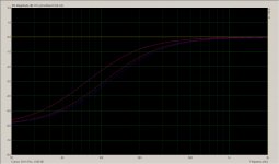
In the attached graph below there are 3 colours:
Purple is a baffle 52cm wide by 90cm high. 115/0.52 gives ~221Hz, however in ARTA the -3dB point is shown as 78Hz.
Red is a baffle 39cm wide by 63cm high. 115/0.39 gives ~295Hz, yet ARTA shows a -3dB point of 105Hz.
Blue is a baffle 29cm wide by 90cm high. 115/0.29 gives ~397Hz, yet ARTA shows a -3dB point of 115Hz.
This is a huge difference from the generally accepted baffle step approximations, so it seems to me there must be some mistake in the calculations ARTA is doing - either a numerical mistake, or an erroneous assumption by the author behind the equations used.
There is quite a bit of information about the baffle step calculator in the following app note:
http://www.fesb.hr/~mateljan/arta/AppNotes/AP4_FreeField-Rev03eng.pdf
Does anyone have any thoughts on this issue ? Have I spotted a major problem or am I somehow confused ?
ARTA has a feature "LF Box diffraction" which is designed to take a near-field measurement of bass response and then apply an estimated correction curve based on the baffle size to estimate the far field response, EG to take into account baffle step, to allow later spicing with a windowed far-field measurement of higher frequencies.
In the documentation it says: "Note: ARTA and STEPS uses the previous expression for the estimation of the diffraction for spherical or rectangular baffled boxes. Some CAD and simulation programs are using a high-frequency geometrical model for the estimation of box diffraction at low frequencies. Such models can give larger errors on low frequencies than the simple model that is presented here."
In other words, it doesn't try to simulate the specific shape of the diffraction curve ripples, taking driver size and positioning into account (like step.exe for example) but rather calculates a smooth idealized 6dB baffle step shelf.
Fair enough, sometimes too much detail in a simulation where accuracy doesn't really exist is a bad thing, however it seems like the corner frequency is still being calculated vastly wrong.
One formula usually given for calculating the half way (3dB) corner point of a 6dB baffle step shift on a rectangular baffle is 115/width in metres. (Technically, the narrowest dimension, which is usually the width)
I noticed that ARTA's results were significantly different from this so I investigated further, calculating 3 different curves using the "LF Box diffraction" overlay feature, using a flat frequency measurement as the starting point to show only the correction curve.
In the attached graph below there are 3 colours:
Purple is a baffle 52cm wide by 90cm high. 115/0.52 gives ~221Hz, however in ARTA the -3dB point is shown as 78Hz.
Red is a baffle 39cm wide by 63cm high. 115/0.39 gives ~295Hz, yet ARTA shows a -3dB point of 105Hz.
Blue is a baffle 29cm wide by 90cm high. 115/0.29 gives ~397Hz, yet ARTA shows a -3dB point of 115Hz.
This is a huge difference from the generally accepted baffle step approximations, so it seems to me there must be some mistake in the calculations ARTA is doing - either a numerical mistake, or an erroneous assumption by the author behind the equations used.
There is quite a bit of information about the baffle step calculator in the following app note:
http://www.fesb.hr/~mateljan/arta/AppNotes/AP4_FreeField-Rev03eng.pdf
Does anyone have any thoughts on this issue ? Have I spotted a major problem or am I somehow confused ?
Attachments
Last edited:
Hi Guy's, sorry I missed these last two posts.
Aucosticraft, the problem I had with the tool was that it only accepted radius for the speaker, for which I didn't have the manufacturers spec for. If it let me put in Sd I'd be a whole lot happier for my vifa's the published spec is Sd but if I try to reverse that to a radius when I use that radius the result I get is different to the result when I use the manual formula. Without accurate specs for both Sd and radius I can't tell if the tool is giving me correct results or whether my method of converting Sd back to radius is flawed
DBmandrake, I've been using the 115/baffle width in meters calculations myself, I haven't read the arta appnote you linked to at this stage, but my guess would be that they are allowing for boundary re-inforcement in their calculations. I'm pretty sure that the 115 formula is for 4 Pi space which is why almost everything I've read suggests using a max of 3db of correction after doing the calculations.
Tony.
Aucosticraft, the problem I had with the tool was that it only accepted radius for the speaker, for which I didn't have the manufacturers spec for. If it let me put in Sd I'd be a whole lot happier
for my vifa's the published spec is Sd but if I try to reverse that to a radius when I use that radius the result I get is different to the result when I use the manual formula. Without accurate specs for both Sd and radius I can't tell if the tool is giving me correct results or whether my method of converting Sd back to radius is flawed DBmandrake, I've been using the 115/baffle width in meters calculations myself, I haven't read the arta appnote you linked to at this stage, but my guess would be that they are allowing for boundary re-inforcement in their calculations. I'm pretty sure that the 115 formula is for 4 Pi space which is why almost everything I've read suggests using a max of 3db of correction after doing the calculations.
Tony.
A small follow up to the original point of this thread - splicing near-field and far field measurements together using ARTA.
[...]
One formula usually given for calculating the half way (3dB) corner point of a 6dB baffle step shift on a rectangular baffle is 115/width in metres. (Technically, the narrowest dimension, which is usually the width)
I noticed that ARTA's results were significantly different from this so I investigated further, calculating 3 different curves using the "LF Box diffraction" overlay feature, using a flat frequency measurement as the starting point to show only the correction curve.
In the attached graph below there are 3 colours:
Purple is a baffle 52cm wide by 90cm high. 115/0.52 gives ~221Hz, however in ARTA the -3dB point is shown as 78Hz.
Red is a baffle 39cm wide by 63cm high. 115/0.39 gives ~295Hz, yet ARTA shows a -3dB point of 105Hz.
Blue is a baffle 29cm wide by 90cm high. 115/0.29 gives ~397Hz, yet ARTA shows a -3dB point of 115Hz.
This is a huge difference from the generally accepted baffle step approximations, so it seems to me there must be some mistake in the calculations ARTA is doing - either a numerical mistake, or an erroneous assumption by the author behind the equations used.
There is quite a bit of information about the baffle step calculator in the following app note:
http://www.fesb.hr/~mateljan/arta/AppNotes/AP4_FreeField-Rev03eng.pdf
Does anyone have any thoughts on this issue ? Have I spotted a major problem or am I somehow confused ?
I've just started to look at this recently.
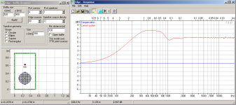
The ARTA application note states (p.5): "For a rectangular box, that has front baffle width w and height h, ARTA currently uses - as an approximation - an equivalent squared box of width d = w*(h/w)^(1/3)."
This is one thing, and you can not compare the outcome of 2 fundamentally different models: yours that takes as sole parameter the width of the baffle, and ARTA's that's also taking the height into account.
Hence with the 1st example you're providing (w = 52 cm, h = 90 cm), ARTA is computing the model of a squared box of width d=62.5 cm.
This model is fully described on the same page. There's the expression of the ratio p4PI/p2PI where f0 has to be substituted by 34.16/d for a squared box.
Below is the computation of this expression for frequencies ranging 10Hz/500Hz, and you can see that indeed the -3dB point is around 78 Hz.

The purpose of this long post is to show that there's no numerical mistake in ARTA. Now, whether their model is erroneous or not is an other question, and I'm not qualified to answer that one.
In my case I'll show the process using the Baffle Diffraction Simulator (BDS) available at the FRD Consortium. Excel required, however.A small follow up to the original point of this thread - splicing near-field and far field measurements...
I wanted to show the process used when I was designing a 2-way with drivers donated by John Krutke (zaph). He had originally given me some SB tweeters to test and later the midwoofers, so I took the time to write a somewhat detailed set of pages on my process, including all files to download and experiment. There's a page that has a number of measurements with two methods of producing a low end, splicing close-mic and using software that extends the response using T/S parameters (CALSOD). The latter has a rudimentary diffraction module, though I never used it. I probably should have.
In my efforts to find a fairly reliable method, I compared the same process using quasi-anechoic large baffle measurements that do not have diffraction to extend the response, extended that with a close-mic large baffle measurement that also has no diffraction, added diffraction to that result and compared it to in-box measurements that do have diffraction coupled with the two methods mentioned.
Zaph hosted the pages. You can see the results by going here and then to the page called "Woofer Close-mic to 4-pi".
There is also a separate page on the BDS results. Jeff Bagby's Diffraction and Boundary Simulator is another option. It will do baffle diffraction on simple geometric baffles. SoundEasy and the new Ultimate Equalizer both have diffraction simulation as well.
At my page, ignore the differences in low end at the tuning frequency. This was a passive radiator design. Some of the measurements have only the woofer response, so the PR system dip is shown. I didn't take the time to combine the woofer and PR responses in this section. The comparison with the CALSOD output is the predicted system response, so it does include both, though rudimentary.
Dave
Does anyone have any thoughts on this issue ? Have I spotted a major problem or am I somehow confused ?
My take on baffle step is that it is a big can of worms and an issue that very very people really understand. I have found that people do not understand why I completely ignore it. Thats because when I take my data it is already present, already accounted for and adding it in again is completely wrong. In fact a lot of people do it wrong.
The one time that it is required is when you have data taken on an infinite baffle and you want to know how that driver will work in a finite box in a free field. Then you need to do some "adjustment", to account for the box diffraction but usually the assumptions made in this adjustment do not hold.
When you use data that was taken in a box of the size that you intend to use, then there is no need to correct for a baffle step, it is already accounted for. And in this last example it is exact, no need of any complex procedures and likely errors.
So to me there is only one situation where this would ever be used and that is not all that common - infinite baffles are rare, so most data does not fit this assumption, and a boxes diffraction more than just the front edge, so in reality a full 3 dimensional model is required. Typically you really do not know how accurate either assumption actually is and it makes a pretty big difference. Its one big giant guess.
My suggestion - never used anyone elses "published" data that claims to be infinite baffle. Measure the actual loudspeaker yourself in a box of similar size and shape as it will be in when complete. Use the actual box when extremely accurate data is required, such as in crossover design.
I have to partly disagree, because for those of us in the DIY community, most measurements that stop at the low end, maybe 300Hz for windowed data, is in the transition region from 2-pi to 4-pi. The diffraction is not taken fully into account. Splicing is often done that does not fully extend the diffraction influence. We see that result as the artificial "hump" in the low end response. That low end data also has poor resolution, further compounding the issue.When you use data that was taken in a box of the size that you intend to use, then there is no need to correct for a baffle step, it is already accounted for. And in this last example it is exact, no need of any complex procedures and likely errors.
Dave
I am not sure that I agree or disagree since I am not sure what part of my comment that you disagree with. The far-field data above the gating frequency, 200-300 Hz is perfectly correct and all diffractions are acounted for. I am not sure on what grounds that you would say that they are not. But when one then goes into the nearfield to take LF data, THEN this data is not really compatible with the far field data because the nearfield diffractions are different than the far field ones. This is going to be particularly true when using a blending freq up arround 300 Hz. So in this sense I can agree with your points.
This problem is not without its resolution however and that is precisely what I am working on now. If one "models" the data as if from a hypothetical sphere then this model is good at all distances from the sphere. Hence I can extrapolate both sets of data, nearfield and midfield, into the same farfield point, usually one that is farther away than either data set was actually taken at. The nearfield LF limited data does not need very many terms to converge (and hence measurement points) because of modal cutof limitiations, usually about three modes/ data points will suffice. The midfield needs more like 16, but that is source dependent. By blending in LF modes only into the first three farfield modes a much more accurate model results than using a single nearfield data point. And it is one in which all diffraction effects are accounted for.
This problem is not without its resolution however and that is precisely what I am working on now. If one "models" the data as if from a hypothetical sphere then this model is good at all distances from the sphere. Hence I can extrapolate both sets of data, nearfield and midfield, into the same farfield point, usually one that is farther away than either data set was actually taken at. The nearfield LF limited data does not need very many terms to converge (and hence measurement points) because of modal cutof limitiations, usually about three modes/ data points will suffice. The midfield needs more like 16, but that is source dependent. By blending in LF modes only into the first three farfield modes a much more accurate model results than using a single nearfield data point. And it is one in which all diffraction effects are accounted for.
I agree with you on this point, it's the data below this point spliced in that is the problem and that was the focus of my post. I see a lot of references to splicing at 500Hz, but I've always felt that this was too high. I prefer 300Hz.I am not sure that I agree or disagree since I am not sure what part of my comment that you disagree with. The far-field data above the gating frequency, 200-300 Hz is perfectly correct and all diffractions are acounted for.
Sounds like an interesting technique. You say you're working on it now. By that I assume that you're creating your own software to do this. I'll be interested in seeing your results if that's so.This problem is not without its resolution however and that is precisely what I am working on now. If one "models" the data as if from a hypothetical sphere then this model is good at all distances from the sphere. Hence I can extrapolate both sets of data, nearfield and midfield, into the same farfield point, usually one that is farther away than either data set was actually taken at. The nearfield LF limited data does not need very many terms to converge (and hence measurement points) because of modal cutof limitiations, usually about three modes/ data points will suffice. The midfield needs more like 16, but that is source dependent. By blending in LF modes only into the first three farfield modes a much more accurate model results than using a single nearfield data point. And it is one in which all diffraction effects are accounted for.
I'm curious about your point that you can extrapolate for other distances with a model. I can see how that can work with an equivalent spherical model. Is it fair to say that you base that on the area below step exhibiting similar characteristics and converging with distance for both sphere and non-sphere of similar response at some specified distance?
The software for diffraction with which I'm familiar will produce results for models at various distances. How is your approach different, other than yours extrapolating from some initial point?
Dave
Is it fair to say that you base that on the area below step exhibiting similar characteristics and converging with distance for both sphere and non-sphere of similar response at some specified distance?
The software for diffraction with which I'm familiar will produce results for models at various distances. How is your approach different, other than yours extrapolating from some initial point?
Dave
I am not sure that I follow the questions.
Consider a sphere that surrounds the actual source. There is some velocity distribution on this sphere that will create an identical far field to an arbitray enclosed source in every way - Thats basically a theorem in acoustics which is based on Greens theorem.
Now fit the data onto this smallish sphere from data at say 2 meters. To within the limits of the models convergence, this data has infinite resolution in both frequency and space. This means that I can go anywhere in the radiation field up to the sphere that I initially assumed - forward or backward.
Now lets say that I take a second data set very close to the assmued sphere. I can extrpolate this data out to say 10 meters and then match it to the midfield data extrapolated out to 10 meters as well. This makes no assumptions about diffraction, etc. at all except that the model has converged. As with most problems, you can track convergence by adding terms. When it doesn't change anymore then it has converged (mostly true, some extreme cases can violate this however).
What is really cool is that you can take the data right down onto the surface of the sphere and plot out the complex velocity response at the surface. This will then show you how the sphere would have had to move to create the measured field. I have used this reconstruction to prove that the axial hole is a result of the waveguides edge diffraction which varies in magnitude depending on whether this frequency has a standing wave across the aperature or not. In the case of the Abbey there is a very pronouced standing wave, while the Summa does not have a standing wave even though it still has the diffraction.
This technique is proving to be extremely powerful and I have not yet decided what to do with it. I am still doing some development, but it is far enough along now that I also use it in my loudspeaker development to find problems, etc. It is what is used to create the extremely hi resolution polar maps that I display.
Righ now it is only valid in the horizontal plane, but the technique is not limted to that, its just that full 3-D adds an imense amount of calculations and data requirements. So I am trying to see how to couple high res horizontal data to low res vertical data to get an ideal combination. It looks like this can be done.
Those well versed in acoustics will recognize this technique as Nearfield Acoustic Holography, or Fourier Acoustics, etc. Not really new, but only recently have computers become powerful enough to do the calcs in a reasonable time frame. Its still a bit much for my laptop, but runs almost in real time on my desktop.
Last edited:
Ah, an enclosing sphere, I misunderstood. This is very clear and interesting. And these are measurements at these points I assume. It's not predictive of something prior to construction, but rather an analysis and extrapolation from measured results, correct?I am not sure that I follow the questions.
Consider a sphere that surrounds the actual source.
Dave
Yes, measurements, sorry if I did not make that clear. Being a strong believer in design by measurements I found that they really weren't as good as they could be. The Farina technique as implimented in Holm was a major breakthrough. The impulse responses that I get now are extremely accurate and high resolution. So it made sense to push the envelope on the analysis side.
A prof at U of M that I know (Weinreich, FYI) wrote a paper back in the 50's showing that with two concentric spheres you could calculate only the source contributions that lie within the spheres. Hence, you could calculate out all of the room reflections. No more LF limit from having to window!
Well that's true in theory. In practice you have to find small differences in two large numbers - the data on the spheres, which at LFs are very similar. This tends to get unstable as the frequency drops. So it remains to be seen if this technique would work any better in practice than windowing. I suspect it would. I do know that I can't move my walls, but maybe I can improve the calculations.
I have to partly disagree, because for those of us in the DIY community, most measurements that stop at the low end, maybe 300Hz for windowed data, is in the transition region from 2-pi to 4-pi. The diffraction is not taken fully into account. Splicing is often done that does not fully extend the diffraction influence. We see that result as the artificial "hump" in the low end response. That low end data also has poor resolution, further compounding the issue.
Dave
Here's how I do it, while retaining phase accuracy.
Dave Dal Farra
Attachments
Your technique does not acount for the diffraction problems that we have been talking about. It maintains phase, yes, but thats all.
What did I miss?
When you blend the nearfield and the far field data how do you account for the fact that the enclosures diffraction effect is different at these two points? Just matching phase won't do that. In fact, I am not so sure that the phase is all that important at these low frequencies.
When you blend the nearfield and the far field data how do you account for the fact that the enclosures diffraction effect is different at these two points? Just matching phase won't do that. In fact, I am not so sure that the phase is all that important at these low frequencies.
I think you read the spreadsheet incorrectly.
Here's the method, your issue doesn't apply: model diffraction at same observation point that the higher frequency quasi anechoic measurement was taken at. Add magnitude of diffraction to the NF measure (dB). Discard phase. Take Hilbert of NF+diffraction. Add in a GD to NF+diffr so that the total GD at the splice frequency equals that of the quasi anechoic measure measure, at the splice frequency.
Phase matters if integrating with subs or if using any xover near or below the splice frequency.
Dave
I didn't read the spreadsheet thats too much work. So it all depends on how accurate the diffraction model is and if you actually need phase integrity. I haven't had the need for the phase, but I think my diffraction model is quite good with my technique.
If you didn't read it, why criticize it?
I posted the diffraction model accuracy earlier, directly compared with anechoic measures. For operation over a narrow range below 300Hz, its good (and enough).
- Status
- This old topic is closed. If you want to reopen this topic, contact a moderator using the "Report Post" button.
- Home
- Loudspeakers
- Multi-Way
- splicing nearfield to farfield, does this look right?