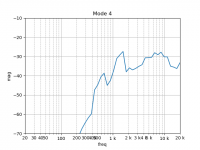
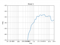
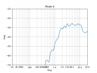
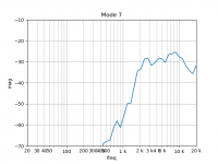
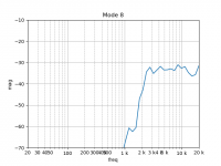
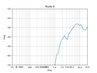
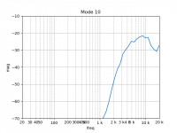
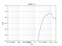
Yes, that is not correct.
I tried to open one of my .txt data files with the app, but it would not open it. Said it was the wrong "type" of file.
if your data is the single file generated by holmimpulse then change filetype to "HolmImpulse" and make sure the header is this format
## sample;0 (H00) ;1 (H05) ;2 (H10) ;3 (H15) ;4 (H20) ;5 (H30) ;6 (H40) ;7 (H50) ;8 (H60) ;9 (H80) ;10 (H100) ;11 (H120) ;12 (H150) ;13 (H180)
i.e. the measurement name is H<angle>
if that doesn't work then pls send me the file and I'll take a look at it to see why it won't open
That didn't work either. All the "open file dialog" shows me are the Holm impulse project files, not the output text files that have the impulse data. The file is too big to attach or I would do that.
Now when I select ".txt" the OPen Dialog tells me that there are no files like that in the directory - but there are.
Last edited:
I replaced line 9 in the file you sent withThat didn't work either. All the "open file dialog" shows me are the Holm impulse project files, not the output text files that have the impulse data. The file is too big to attach or I would do that.
Now when I select ".txt" the OPen Dialog tells me that there are no files like that in the directory - but there are.
## sample;0 (H00) ;1 (H05) ;2 (H10) ;3 (H15) ;4 (H20) ;5 (H30) ;6 (H40) ;7 (H50) ;8 (H60) ;9 (H80) ;10 (H100) ;11 (H120) ;12 (H150) ;13 (H180)
and saved
then
- open pypolarmap
- click load measurements
- change dropdown to HolmImpulse
- click Select File(s)
- select the edited file
- measurements are loaded
if the above process does not work for you then that's confusing
anyway I put the window as follows, is this ok?
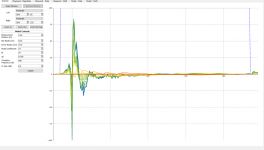
this results in
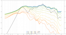
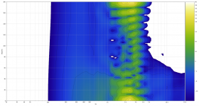
Ok, I can open the file now.
1) The window is extremely hard to set. In my code you just drag a line and set the window - done. Only one impulse should be shown - the axial - as this will determine the correct window length.
2) The modal fit is certainly wrong.
3) a line on the polar map showing the angle for the top plot would be almost essential. Another line showing the frequency would also be nice. Its very hard to tell what the angle and frequency are.
What I would need to see to debug the error is a plot of Modal coefficients versus frequency.
yes there are certainly some usability enhancements required, happy to tackle thoose once it is actually working properly
"extremely hard to set" seems a bit strong mind you
* load measurements
* click find first peak
* click zoom in
* change value in right or left manually then click zoom in again
* repeat til the window is where you want it
* click apply window
not the easiest or most intuitive but not what I'd call hard either
What I would need to see to debug the error is a plot of Modal coefficients versus frequency.
it's been a little while since I looked at this code so can you confirm exactly which data you want pls?
is it just the data returned from CalSpatial?
"extremely" might be a bit strong. It's a lot of steps compared to "click" just before first reflection and then "set window". I don't see why it needs to be more complicated than that. The first reflection is almost always going to be in the first 500-700 data points, so showing more than that is not helpful.
In my data set the "find first peak" wasn't even close to the first reflection. The code said 200 something and the first reflection was at about 327.
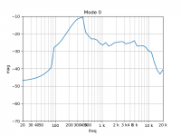
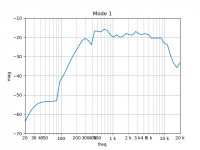
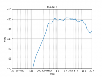
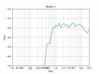
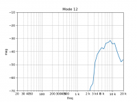
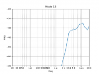
Yes, I need to see the array ModalData(,) output from CalcSpatial, plotted as magnitude versus frequency for the number of modes calculated (or say the first ten.) There are some strange single point dropouts of -30 dB that can't be real in the results.
It also appears to me that the polar map is going from 0 - 360 and not 0 - 180. I'd prefer 0 - 90 as thats the data that we really want to see. The rear stuff is not very interesting.
well tbh the answer (to why it is clunky) is because, at the time I wrote this, I didn't know how to implement an interactive chart using this lib without it being really v slow (matplotlib is v capable but interactivity is not the strong suit). I've written another qt/matplotlib app since then which means I now have a better handle on how to do this now so expect to be able to sort that out
fwiw the find first peak is just scipy.signal.find_peaks_cwt — SciPy v1.1.0 Reference Guide
it's obviously sensitive to the shape of the signal but has worked well for some data I've tried it on, not so well for some other data. I imagine it's unlikely there is one set of parameters that works well for all measurements and the human brain/eye will do a better job more quickly so I expect that will be dropped once I write a friendlier screen for setting the window.
anyway I'll generate that data for you
Thanks, and I do appreciate your diligence and participation. Let's make this something valuable.
PS. I am now not so sure that we can't exclude room reflections while rotating the source. I need to review the Weinreich paper and perhaps even talk with him since he lives just a few miles from me. I don't actually know him, but I would love the chance to talk with him about this.
PS. I am now not so sure that we can't exclude room reflections while rotating the source. I need to review the Weinreich paper and perhaps even talk with him since he lives just a few miles from me. I don't actually know him, but I would love the chance to talk with him about this.
I had the app running and lowered it to the taskbar. A few hours later came back and it was frozen. FYI
Also, I would need to see these same plots within the app - on a tab (which can be hidden later)- while I do some things. That way I can debug what is going on i.e. what ka value does mode 0 go bad and does this vary with field location or with the assumed source radius, etc. ... critical to know these things.
PS it's actually not so bad that the error is going to be simple. You appear to be interacting correctly with the DLL, but something is amiss.
Last edited:
try this build - Release Display modal parameters * 3ll3d00d/pypolarmap * GitHubAlso, I would need to see these same plots within the app - on a tab (which can be hidden later)- while I do some things. That way I can debug what is going on i.e. what ka value does mode 0 go bad and does this vary with field location or with the assumed source radius, etc. ... critical to know these things.
the window controls are hopefully a bit more user friendly and the modal response in the new modal - parameters tab. There is a glitch with the multi view charts in that leaving the tab and going back to it stops the chart working.
if you hit ctrl+m then you should be able to tweak the modal parameters and see the results
if you hit ctrl+l (while focus is on the main window) and put that into DEBUG then you'll see the parameters (excluding the actual data as I thought that would be a bit too much info) passed into the various function calls.
let me know if you need anything else in order to be able to debug further
At this point, below 200 Hz is pretty well meaningless. We will need to add in some further techniques for that area, but above 200 Hz what you are showing looks exactly correct.
I think that I might have found the problem. When I "commented out" the LF fitting stuff I may have to correct the remainder. I was never completely happy with my LF fit - I could always get it to work, but it took too much human interaction and it only worked well for monopoles. When we decided to do this work I commented out all that stuff to focus on just the higher frequency range, but might not have completely left behind correct code.
I need to do some further tests.
My son works in the Physics Dept. at UM, where Weinreich is an Emeritus Prof. I am trying to get in touch with him to discuss my ideas for using two different radius measurements to exclude external reflections, but still allow for the source to be rotated and the mic stationary. I now believe that, in theory, this should be possible.
Last edited:
- Home
- Design & Build
- Software Tools
- Klippel Near Field Scanner on a Shoestring
