That being said, if we rely on IR gating to measure as low as possible before using field separation, the frequency resolution will be, as I'm sure you know, quite low and any lower frequency anomalies would be very blurred or invisible. Having better than +200Hz resolution below 500Hz-1kHz seems beneficial.
Just to be clear, I would suggest using a 200 Hz gate only above 200 Hz and use a much longer time window for data below 200 Hz and the dual radius technique to cancel the incoming reflection out of the data. This would yield far more resolution at LFs than would actually be required at these LFs (because our hearing has low LF resolution anyways.) This is another reason why the data being transferred into our analysis software should not be gated as we would use different gates for different frequency regions.
If a two layer scan were done then the LFs could be cleared of reflections and the HFs could be fitted at the two different radii and averaged for an improvement in both frequency regions.
If one were only really interested in > 200 Hz, like myself, they could simply skip the second layer.
starting to make some sort of progress with a UI though I haven't put any effort into making it look pretty so ignore the fact the layout is a bit rough 
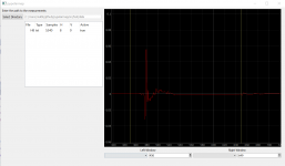
this can load measurements from a folder and display n impulses in a chart, the chart widget has built in mouse controls for panning and zooming and it seems to move v smoothly. I've added draggable lines (the yellow lines shown) and these are connected to the spinners below (so dragging updates the value in the spinner as well as updating the spinner moves the line) to verify that I can handle user interaction with the chart and determine things like where they clicked or what moved where.
Code is visible at pypolarmap/src/python at wrapper * 3ll3d00d/pypolarmap * GitHub if anyone wants to poke around
I think the next steps are
- use those markers to create windows
- allow the user to see the windowed IRs
- feed that into the fft & lintolog functions from the @gedlee's dll
- plot those results
Just to be clear, I would suggest using a 200 Hz gate only above 200 Hz and use a much longer time window for data below 200 Hz and the dual radius technique to cancel the incoming reflection out of the data.
...
If a two layer scan were done then the LFs could be cleared of reflections and the HFs could be fitted at the two different radii and averaged for an improvement in both frequency regions.
Agreed.
If one were only really interested in > 200 Hz, like myself, they could simply skip the second layer.
I think for the first iteration of this, skipping <200Hz is fine. But I'd like to eventually get to the point where we could do sound field separation and get down to ~20Hz.
And hoping this actually goes somewhere. Firstly to be able to do this kind of measurement on a budget.
Me too!
starting to make some sort of progress with a UI though I haven't put any effort into making it look pretty so ignore the fact the layout is a bit rough
View attachment 690204
this can load measurements from a folder and display n impulses in a chart, the chart widget has built in mouse controls for panning and zooming and it seems to move v smoothly. I've added draggable lines (the yellow lines shown) and these are connected to the spinners below (so dragging updates the value in the spinner as well as updating the spinner moves the line) to verify that I can handle user interaction with the chart and determine things like where they clicked or what moved where.
Code is visible at pypolarmap/src/python at wrapper * 3ll3d00d/pypolarmap * GitHub if anyone wants to poke around
I think the next steps are
- use those markers to create windows
- allow the user to see the windowed IRs
- feed that into the fft & lintolog functions from the @gedlee's dll
- plot those results
Looks like a great start to me!
starting to make some sort of progress with a UI though I haven't put any effort into making it look pretty so ignore the fact the layout is a bit rough
Lookin good. I'm following you on Github as well. This is a great idea.
starting to make some sort of progress with a UI though I haven't put any effort into making it look pretty so ignore the fact the layout is a bit rough
Good start. I looked at the code and as expected could not make head or tails out of it except that it appears to rely on a great deal of imported resources. Hence I guess that you need to understand those resources.
And good luck to England, but my money is on Brazil.
Last edited:
I think for the first iteration of this, skipping <200Hz is fine. But I'd like to eventually get to the point where we could do sound field separation and get down to ~20Hz.
I agree. Once we have a useful app that is simplified down to the lowest but still usable level, then it only makes sense to add in more and more capability - but down the road, not at this stage.
I added the gate & window which you can see in pypolarmap/impulse.py at wrapper * 3ll3d00d/pypolarmap * GitHub
this is my interpretation of how something like ARTA or REW applies a window, never implemented such a thing before so appreciate it if someone can give it the once over. The resulting graphs look sane so it seems ok to me.
now to feed that into the fft and plot the result
this is my interpretation of how something like ARTA or REW applies a window, never implemented such a thing before so appreciate it if someone can give it the once over. The resulting graphs look sane so it seems ok to me.
now to feed that into the fft and plot the result
I added the gate & window which you can see in pypolarmap/impulse.py at wrapper * 3ll3d00d/pypolarmap * GitHub
this is my interpretation of how something like ARTA or REW applies a window, never implemented such a thing before so appreciate it if someone can give it the once over. The resulting graphs look sane so it seems ok to me.
now to feed that into the fft and plot the result
Your Notes in the coding are awesome.
My last brush with programming was via Turbo PASCAL as my high level programming language many moons ago. I can actually figure out what you are doing. Numpy is doing the heavy lifting I'm guessing?
if anyone wants to run this then I think this should do the job
- download and install the 32bit anaconda -> Downloads - Anaconda
- open an anaconda shell and
note that very specific versions are listed there because the latest versions seem flaky (I hit the same problem mentioned in this issue as soon as I import numpy)
- I use jetbrains IDEs so download pycharm community -> https://www.jetbrains.com/pycharm/download/#section=windows
- install it and use it to clone my repo from github
- set the project interpreter to the python.exe in your scanner32 environment (so by default this will be c:\Users\<username>\Anaconda3\envs\scanner32\python.exe)
- open the directory (containing the source) as a pycharm project then create a run config to run app.py
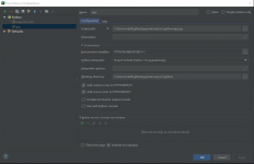
- run it and away you go
note that it currently only reads files that are basically wavs in txt form (i.e. a txt file containing a load of floats, 1 per line) and also doesn't do much except stick them on screen but I thought I might as well post this anyway
- download and install the 32bit anaconda -> Downloads - Anaconda
- open an anaconda shell and
Code:
conda create -name scanner32 python=3.6 numpy=1.14.3 mkl=2018.0.2
conda activate scanner32
conda install pyqtgraph scipy
note that very specific versions are listed there because the latest versions seem flaky (I hit the same problem mentioned in this issue as soon as I import numpy)
- I use jetbrains IDEs so download pycharm community -> https://www.jetbrains.com/pycharm/download/#section=windows
- install it and use it to clone my repo from github
- set the project interpreter to the python.exe in your scanner32 environment (so by default this will be c:\Users\<username>\Anaconda3\envs\scanner32\python.exe)
- open the directory (containing the source) as a pycharm project then create a run config to run app.py

- run it and away you go
note that it currently only reads files that are basically wavs in txt form (i.e. a txt file containing a load of floats, 1 per line) and also doesn't do much except stick them on screen but I thought I might as well post this anyway
added an initial rendering of the FR using @gedlee's fft and linToLog functions
pypolarmap/magnitude.py at wrapper * 3ll3d00d/pypolarmap * GitHub
using the previously written python wrapper
pypolarmap/__init__.py at wrapper * 3ll3d00d/pypolarmap * GitHub
I'd include a screenshot but it is very very crashy atm so I can't. fft is fine but linToLog either crashes on call or succeeds and then the python process dies soon after with an error code that indicates a heap corruption. I think this implies I'm feeding it data it doesn't expect and/or can't cope with.
On the odd occasion I've seen the resulting chart, I'd say the raw fft data looks much like the FR produced by REW (so I think this backs up the above, this is working fine) while the linToLog looks a bit unstable at the low end (i.e. FR oscillates up and down)
I'm not sure how to work this out, @gedlee any ideas? I can translate the python code into pseudocode if you think that would help.
I think mine probably is too but we live in hope!And good luck to England, but my money is on Brazil.
Last edited:
Your Notes in the coding are awesome.
+1
very nice clean coding!
in pseudo code for a single measurement, my test measurement is some random in room measurement at 48kHz with a 1st reflection at about 3.5ms (i.e. about 170 samples)
- apply gate (e.g. left 25 samples, right 175 samples == 200 sample wide gated measurement)
- apply window (e.g. hann 50%)
- this gives you a set of samples as follows
in pictures
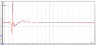
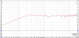
now pass this to the dll
- zero pad to a power of 2 sized array (e.g. append 56 zeroes to make the input data 256 long)
- pass into the fft function and return 2 results from this function
1) an array of complex numbers (e.g. there will be 128 complex numbers)
2) the no of samples passed into the fft (e.g. 256)
- pass the results into the linToLog function which has the following arguments
1) FFT data = the array of 128 complex numbers we got from the fft
2) DeltaF = fs / fftSize = 48000/256 = 187.5
3) inputPts = length of 1) = 128
4) outputPts = a writeable array of 128 complex numbers initialised with zeroes
5) logPoints = length of 6) = 128
6) freqs = an array of double precision values initialised with n erb spaced frequencies from 20-24000Hz (I had this hardcoded to 200 earlier but it's now min(200, inputPts))
the erb freqs are calculated using an algorithm I copied from brian/erb.py at 2ac30d709d3d47020eda7a4e9e51854c0577f7b2 * brian-team/brian * GitHub
the result of the above is something that generally can complete the call to the function but that crashes the process soon after with a heap corruption sort of behaviour
what I think I need to work out is whether I'm calling it incorrectly (i.e. the data is incorrect) or whether the way I'm calling it is incorrect (i.e. the python-fortran bridge is incorrectly defined in some way)
If we can confirm the input data is valid then I can concentrate on the 2nd aspect.
- apply gate (e.g. left 25 samples, right 175 samples == 200 sample wide gated measurement)
- apply window (e.g. hann 50%)
- this gives you a set of samples as follows
Code:
[-0.00000000e+00  2.73620395e-07 -7.61226994e-07 -2.52245891e-06
  4.93732512e-06 -9.00115774e-06  1.68079168e-05 -3.19783513e-05
  2.00698027e-05 -2.38814257e-05 -2.17229128e-05  6.11723060e-05
 -8.80999800e-05  3.28894240e-04  3.32448780e-04  5.25968000e-04
 -1.56762610e-03 -2.39794080e-04  4.87322580e-05 -6.95903360e-05
  2.54811840e-04 -9.58889660e-04 -8.37712200e-03 -3.43294000e-02
  1.12837140e-02  5.56975400e-02  5.07188700e-03 -5.53199740e-03
  2.87325450e-03 -1.06123750e-02 -5.38069400e-03 -7.68214370e-03
 -8.36833800e-03 -4.80978400e-03 -5.42689670e-03 -2.24059120e-03
 -4.11024600e-03 -1.01462440e-03  4.07823860e-04 -4.00713240e-04
  5.94695160e-04 -5.34936100e-04  4.63901200e-03  6.78018850e-03
  3.54289170e-03  3.51933530e-03  2.30075470e-03  6.08390600e-04
  3.58891000e-03  5.72224500e-03  5.25780600e-03  6.03630670e-03
  4.95591430e-03  1.82186180e-03  2.26518370e-03  2.31504250e-03
  2.07585470e-03  3.29644930e-03  3.40835540e-03  2.06255630e-03
  1.70133300e-03  7.43033500e-04  3.34356200e-04  2.71687330e-03
  2.27495380e-03 -6.82341340e-05  3.32759840e-04  1.21086560e-03
  1.24475230e-03  1.20506690e-03  8.48432250e-04  6.25180300e-04
  3.63202470e-04 -5.69753640e-04 -1.65841160e-04 -6.36112640e-04
 -1.90886740e-03 -5.58558740e-04 -2.17195960e-05 -5.72648830e-04
 -8.32985970e-04 -1.23660030e-03 -1.12132570e-03 -1.19920480e-03
 -1.24329330e-03 -8.38635660e-04 -6.26191030e-04 -5.12037300e-04
 -3.83403600e-04 -2.71916300e-04 -2.34764610e-04 -1.53737200e-04
 -2.77250130e-04 -6.93635670e-04 -6.60004440e-04 -4.21458100e-04
 -3.68384940e-04 -1.30858560e-04 -3.73437420e-04 -7.57266400e-04
 -6.20050500e-04 -6.81405650e-04 -7.27064730e-04 -5.93181100e-04
 -7.11710900e-04 -8.16094000e-04 -7.62677640e-04 -7.77286000e-04
 -8.69720940e-04 -7.92722700e-04 -7.28134300e-04 -8.03075150e-04
 -7.53068693e-04 -8.95815518e-04 -1.05186019e-03 -8.51176855e-04
 -6.35659754e-04 -5.57582275e-04 -6.34001894e-04 -8.04708840e-04
 -8.76975416e-04 -7.73103300e-04 -6.80853801e-04 -7.25804201e-04
 -7.03933904e-04 -6.28786579e-04 -5.79931543e-04 -5.73622575e-04
 -6.38869679e-04 -6.31387363e-04 -5.42402043e-04 -4.32172266e-04
 -3.97643739e-04 -4.68533088e-04 -4.76440667e-04 -4.07618700e-04
 -3.63935215e-04 -3.30481725e-04 -3.48059098e-04 -3.95638007e-04
 -3.61284089e-04 -2.93341168e-04 -2.92648134e-04 -3.07025031e-04
 -2.70489535e-04 -2.73217213e-04 -2.70793168e-04 -2.40275637e-04
 -2.69844524e-04 -2.83528424e-04 -2.68908182e-04 -2.75242597e-04
 -2.60368305e-04 -2.42501217e-04 -2.46651283e-04 -2.47133073e-04
 -2.24474157e-04 -2.30721761e-04 -3.19663003e-04 -1.86296681e-04
 -6.43799099e-05 -2.83230199e-04 -3.37111732e-04 -2.28424430e-04
 -2.27834475e-04 -2.27880582e-04 -2.27555542e-04 -2.43754161e-04
 -1.41830779e-04 -5.17271891e-05 -1.54469333e-04 -1.99855181e-04
 -1.47463841e-04 -1.19121511e-04 -8.83055121e-05 -1.17039523e-04
 -1.10197218e-04 -5.60569378e-05 -7.17032875e-05 -9.76294222e-05
 -8.92865994e-05 -5.60927451e-05 -3.52839667e-05 -3.00747922e-05
 -1.88561339e-05 -1.30092928e-05 -1.04228997e-05 -1.10665068e-05
 -1.10842691e-05 -8.61607914e-06 -1.08527619e-05 -7.40856438e-06
 -4.48033874e-06 -2.98474555e-06 -9.75631864e-07 -8.99298601e-07
 -2.34399622e-06 -2.81809951e-06 -2.04474322e-07  0.00000000e+00]
in pictures


now pass this to the dll
- zero pad to a power of 2 sized array (e.g. append 56 zeroes to make the input data 256 long)
- pass into the fft function and return 2 results from this function
1) an array of complex numbers (e.g. there will be 128 complex numbers)
2) the no of samples passed into the fft (e.g. 256)
- pass the results into the linToLog function which has the following arguments
Code:
    # COMPLEX(8), intent(in):: DataIn(0:NumFFTPts)        ! FFT data in at all angles
    # real(8), intent(in) :: DeltaF                      ! the frequency delta
    # integer, intent(in):: NumFFTPts                    ! the number of FFT points in the input
    # COMPLEX(8), intent(out) :: DataOut(0:NumLogPts)    ! The interpolated log frequency output
    # integer, intent(in) :: NumLogPts                   ! number of smoothed output points ‐ log scaled
    # real(8), intent(out) :: Freqs(0:NumLogPts)          ! the Array of output frequencies
1) FFT data = the array of 128 complex numbers we got from the fft
2) DeltaF = fs / fftSize = 48000/256 = 187.5
3) inputPts = length of 1) = 128
4) outputPts = a writeable array of 128 complex numbers initialised with zeroes
5) logPoints = length of 6) = 128
6) freqs = an array of double precision values initialised with n erb spaced frequencies from 20-24000Hz (I had this hardcoded to 200 earlier but it's now min(200, inputPts))
the erb freqs are calculated using an algorithm I copied from brian/erb.py at 2ac30d709d3d47020eda7a4e9e51854c0577f7b2 * brian-team/brian * GitHub
the result of the above is something that generally can complete the call to the function but that crashes the process soon after with a heap corruption sort of behaviour
what I think I need to work out is whether I'm calling it incorrectly (i.e. the data is incorrect) or whether the way I'm calling it is incorrect (i.e. the python-fortran bridge is incorrectly defined in some way)
If we can confirm the input data is valid then I can concentrate on the 2nd aspect.
First, the frequency spacing should be true log and not ERB. In my code it looks like:
For ifreq = 0 To system_.NumLogPts - 1
Freqs(ifreq) = IFreqToFreqs(ifreq)
Next ifreq
End Sub
Public Function IFreqToFreqs(ByVal ifreq As Integer) As Double
Return 2.0 * Math.Pow(10.0, LOWEST_DEC + NUMBER_DEC * ifreq / (system_.NumLogPts - 1))
End Function
Also, having too few FFT points may be a problem, I'm not sure, but I would certainly not fit log points to the same number as linear points as this would not likely yield very good results. The lowest number of FFT points that I have used is 512 and the highest number of linear points is 200. Outside of that range and the code has never been tested.
The FFT data would actually be 129 complex numbers right? Not 128 (0:128 is 129 points). Recall that you must unwrap the output of FFT to yield n/2 + 1 complex points. If this was not done then it will really mess things up.
Beyond that I can't offer up much help. This is precisely why I was so concerned with the GUI being done in a manner which I cannot duplicate.
Also, regarding the window, I use a flat window with gradual taper only at the very end of the window. A fairly sharp cosine taper to zero over the last few ms. There are better ways to do this, but I have never taken the time to implement them since the above window worked just fine. The Hann window would not be appropriate here.
The FFT data would actually be 129 complex numbers right? Not 128 (0:128 is 129 points). Recall that you must unwrap the output of FFT to yield n/2 + 1 complex points. If this was not done then it will really mess things up.
Beyond that I can't offer up much help.
This seems to be progressing well I wish I could help but I just don't have the bandwidth to do more that cheer from the sidelines.
The numbers thing is just bookkeeping, there is simply a language dependent convention, for Python a range of 0 to 128 has 128 elements. IIRC Fortran had 1 as the first index of an array (which to me never made any sense).
ok apologies I misunderstood and/or missed your previous message.the frequency spacing should be true log and not ERB
in python/numpy terms, this is just
Code:
np.logspace(math.log10(20), math.log10(20000), num=numLogPts, endpoint=True)512 points equates to a ~10ms gate in the absence of zero padding which implies a minimum of ~5ms with zero padding to a power of 2 sized array. If we're placing that sort of lower bound on the measurement setup then that seems a key thing to note. Is that what you mean by this?The lowest number of FFT points that I have used is 512
ok I'm doing this wrong as well. You previously said:The FFT data would actually be 129 complex numbers right? Not 128 (0:128 is 129 points). Recall that you must unwrap the output of FFT to yield n/2 + 1 complex points. If this was not done then it will really mess things up.
the 0 point and the N+1 complex data are returned in the first complex number as real(0) as the real part and real(N+1) as the complex part.
The complex part of both these points must be zero (guaranteed.)
As I said before, the FFT is an array of N/2 + 1, and the zeroth element is the real part of the first element in the array passed out and the real part of the N/2+1 element is is the imaginary part of the zeroth element.
so lets say we have a float64 array with 512 values (i.e. a load of double precision samples), I pass that into your function and the array is still 512 float64 values into which is packed 257 complex128 values. Call this A and call the intended complex128 output X then
A[0] == X[0]+0i
A[1] == X[257]+0i
A[2:].view(complex128) == X[2:257]
i.e.
1st float64 is 1st complex output (with 0i assumed)
2nd float64 is last complex output (with 0i assumed)
view the remainder as complex and you get another 255 complex numbers
if this is correct then I've done this and it's still crashy. It does not crash all the time though and it is crashing when the data in the output area is read by python code (i.e. if I don't touch that array then the program is stable). This certainly confirms the output data contains something "bad" but what and why is another question.
I don't think this is that big a concern really, it's just a question of being able to specify the behaviour of the functions in the DLL. If we can do this then writing a gui is not so hard and working out how to drive the dll should not be that hard.This is precisely why I was so concerned with the GUI being done in a manner which I cannot duplicate.
I put tukey as an option so that seems like it should do, do you agree?Also, regarding the window, I use a flat window with gradual taper only at the very end of the window. A fairly sharp cosine taper to zero over the last few ms. There are better ways to do this, but I have never taken the time to implement them since the above window worked just fine. The Hann window would not be appropriate here.
Last edited:
in python/numpy terms, this is just
Code:np.logspace(math.log10(20), math.log10(20000), num=numLogPts, endpoint=True)
See, I can't follow that as there is just not enough information.
512 points equates to a ~10ms gate in the absence of zero padding which implies a minimum of ~5ms with zero padding to a power of 2 sized array. If we're placing that sort of lower bound on the measurement setup then that seems a key thing to note. Is that what you mean by this?
I just take the data and whereever the window is set to place data and beyond that zeros. I don't see what a power of two has to do with it.
ok I'm doing this wrong as well. You previously said:
so lets say we have a float64 array with 512 values (i.e. a load of double precision samples), I pass that into your function and the array is still 512 float64 values into which is packed 257 complex128 values. Call this A and call the intended complex128 output X then
A[0] == X[0]+0i
A[1] == X[257]+0i
A[2:].view(complex128) == X[2:257]
i.e.
1st float64 is 1st complex output (with 0i assumed)
2nd float64 is last complex output (with 0i assumed)
view the remainder as complex and you get another 255 complex numbers
if this is correct then I've done this and it's still crashy. It does not crash all the time though and it is crashing when the data in the output area is read by python code (i.e. if I don't touch that array then the program is stable). This certainly confirms the output data contains something "bad" but what and why is another question.
I put tukey as an option so that seems like it should do, do you agree?
I don't know "tukey" as a window and at any rate there is no name for the window I use, but it is logically derived to yield the best data for fitting.
I can't follow your explanations about the arrays. I don't understand
A[2:].view(complex128) == X[2:257]
but to me that is 257 points which is correct
Last edited:
- Home
- Design & Build
- Software Tools
- Klippel Near Field Scanner on a Shoestring