4P1L Triode Connection
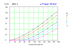
Just received 4 NOS 4P1L in addition to ones I had on hand. I curved all of them in triode connection and also generated a model in uTgui.
Again the caveat is this model was created from an actual and only single tube.. I guess I could create a bunch of models and average the values of a bunch of them to create an "average" device model. Hmmm..
* n* library format: LTSpice
* Traced by Kevin Kennedy 2014-04-18 in uTgui
* Unselected sample
.SUBCKT 4P1L-TRI 1 2 3 ; P G C (Triode)
X1 1 2 3 TRIODE MU=10.25 EX=1.48 KG1=1177.7 KP=631.61 KVB=376.5 VCT=0.00 RGI=2000 CCG=0p CPG1=0p CCP=0p ;
.ENDS 4P1L-TRI
Interesting how well three of these four samples match each other, and even the odd one out is not that far off.
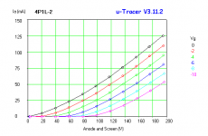
Attachments

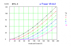
Again the caveat is this model was created from an actual and only single tube.. I guess I could create a bunch of models and average the values of a bunch of them to create an "average" device model. Hmmm..
If the model behaves similar (+-20%) to the datasheet, then it's ok, otherwise, it is probably not so useful to the others - that's the only downside I see with using uTgui to generate the models - that they become "one-offs".
5902 Pentide Model
Code:
*
* Generic pentode model: 5902_AN
* Copyright 2003--2008 by Ayumi Nakabayashi, All rights reserved.
* Version 3.10, Generated on Sat Apr 19 08:35:34 2014
*               Plate
*               | Screen Grid
*               | |  Control Grid
*               | |  |  Cathode
*               | |  |  |
.SUBCKT 5902_AN A G2 G1 K
BGG   GG   0 V=V(G1,K)+0.99999999
BM1   M1   0 V=(0.14268581*(URAMP(V(G2,K))+1e-10))**-1.3148991
BM2   M2   0 V=(0.53287878*(URAMP(V(GG)+URAMP(V(G2,K))/3.2737748)))**2.8148991
BP    P    0 V=0.0012595553*(URAMP(V(GG)+URAMP(V(G2,K))/6.1435638))**1.5
BIK   IK   0 V=U(V(GG))*V(P)+(1-U(V(GG)))*0.0010592697*V(M1)*V(M2)
BIG   IG   0 V=0.00062977765*URAMP(V(G1,K))**1.5*(URAMP(V(G1,K))/(URAMP(V(A,K))+URAMP(V(G1,K)))*1.2+0.4)
BIK2  IK2  0 V=V(IK,IG)*(1-0.4*(EXP(-URAMP(V(A,K))/URAMP(V(G2,K))*15)-EXP(-15)))
BIG2T IG2T 0 V=V(IK2)*(1.0088853952*(1-URAMP(V(A,K))/(URAMP(V(A,K))+10))**1.5+-0.0088853952)
BIK3  IK3  0 V=V(IK2)*(URAMP(V(A,K))+850)/(URAMP(V(G2,K))+850)
BIK4  IK4  0 V=V(IK3)-URAMP(V(IK3)-(0.00094950212*(URAMP(V(A,K))+URAMP(URAMP(V(G2,K))-URAMP(V(A,K))))**1.5))
BIP   IP   0 V=URAMP(V(IK4,IG2T)-URAMP(V(IK4,IG2T)-(0.00094950212*URAMP(V(A,K))**1.5)))
BIAK  A    K I=V(IP)+1e-10*V(A,K)
BIG2  G2   K I=URAMP(V(IK4,IP))
BIGK  G1   K I=V(IG)
* CAPS
CGA   G1  A  0.2p
CGK   G1  K  4.5p
C12   G1  G2 3p
CAK   A   K  8.5p
.ENDSThank you Kevin.
Last year bought 8 pieces 4P1L. All tubes looks like new.
Have no tracer around. I made a triode circuit and measuring current of each tube. Ik ranged from 21.3 mA to 21.8 mA. Each tube has been given a 15-minute DC preheating.
It seems almost a perfectly. I was very surprised by the results. Some esteemed manufacturers could not boast such.
I started breadboard C3m - step down IT - PSE 4P1L. We'll see how it will be at higher current.
Hey Rajko,
That sounds like a very interesting build for the 4P1L in PSE. You may want to try the model I developed for 4P1L with A2 grid current. This will give you a great insight on the PSE operation when optimising your C3m driver:
4P1L model improved | Bartola Valves
Cheers, Ale
That sounds like a very interesting build for the 4P1L in PSE. You may want to try the model I developed for 4P1L with A2 grid current. This will give you a great insight on the PSE operation when optimising your C3m driver:
4P1L model improved | Bartola Valves
Cheers, Ale
Convergence Friendly Tube Models
Hello,
This message is about how to write tube models that are "convergence friendly" in LTspice. This advice probably applies to all SPICE type simulators, although I have not tested this technique in anything but LTspice.
A good model will not only match the typical operational curves of the data sheet reasonably well, but it will also be well behaved for all numerically possible operating conditions, even ones never likely to be normally encountered in a physical circuit. This is because these extreme operating points may fall within the exploratory range of the simulation engine as it searches for the actual operational solution and these extremes must not lead to divergent or latching trial solutions (which then may lead to the dreaded "time step too small" error message and an aborted simulation).
LTspice will have the least trouble achieving a solution with models that describe a current that is a continuous function of voltage with a continuous first derivative of that function with respect to voltage. Note that I stated current as function of voltage. LTspice, like all SPICEs, performs best with voltage controlled current sources. Unfortunately, it seems people have a strong preference for thinking in terms of voltage sources. And it is when behavioral voltage sources are used to define highly nonlinear tube behavior that the simulator is set up to potentially fall into a convergence trap.
LTspice uses Modified Nodal Analysis to process Thevenin type devices such as voltage sources, but this slows down the simulation about as much as adding two Norton type devices such ideal capacitors, resistors or current sources. However, this minor computational bloat is not the reason why nonlinear voltage sources can be so problematic.
Whenever the simulator reduces the time step, it is because of nonlinear circuit behavior. The implicit assumption is that, as the time step is reduced, the various parasitic and stray capacitances will come to dominate the nonlinear bits (which don't depend on time). At really small time steps, only the capacitances will matter and, since capacitances are linear, the circuit will converge to within the error tolerances and the simulator will be able to get past the nonlinear behavior. It can't be stressed enough that stiff voltage sources (especially nonlinear behavioral types) are problematic because, unlike current sources and/or resistors, they will not yield to capacitances at small time steps during convergence difficulties in a transient analysis.
Here is an example of a common tube model that follows these techniques:
Note that the first thing the model does is to translate all the electrode voltages to be ground referenced with a grounded cathode internal model so that the model equations can be simplified with no need to express voltages differentially with respect to the cathode. This probably speeds up the internal math a small amount, but it mainly makes writing the equations much more straightforward. However, the main reason for taking this step is to decouple the terminal voltages from depending on the nonlinear tube equations if the simulator must vastly reduce the time step because of convergence problems. Note that the convergence decoupling time constant is 1ns, a value that should not interfere in any way with the "low frequency" behavior of the model.
Here is an example of a slightly more complex model (no need for comments - same techniques are used):
Note that the behavioral expressions in both models limit current gracefully when the model is heavily overdriven (such as would likely be experienced in a guitar amplifier simulation).
Hello,
This message is about how to write tube models that are "convergence friendly" in LTspice. This advice probably applies to all SPICE type simulators, although I have not tested this technique in anything but LTspice.
A good model will not only match the typical operational curves of the data sheet reasonably well, but it will also be well behaved for all numerically possible operating conditions, even ones never likely to be normally encountered in a physical circuit. This is because these extreme operating points may fall within the exploratory range of the simulation engine as it searches for the actual operational solution and these extremes must not lead to divergent or latching trial solutions (which then may lead to the dreaded "time step too small" error message and an aborted simulation).
LTspice will have the least trouble achieving a solution with models that describe a current that is a continuous function of voltage with a continuous first derivative of that function with respect to voltage. Note that I stated current as function of voltage. LTspice, like all SPICEs, performs best with voltage controlled current sources. Unfortunately, it seems people have a strong preference for thinking in terms of voltage sources. And it is when behavioral voltage sources are used to define highly nonlinear tube behavior that the simulator is set up to potentially fall into a convergence trap.
LTspice uses Modified Nodal Analysis to process Thevenin type devices such as voltage sources, but this slows down the simulation about as much as adding two Norton type devices such ideal capacitors, resistors or current sources. However, this minor computational bloat is not the reason why nonlinear voltage sources can be so problematic.
Whenever the simulator reduces the time step, it is because of nonlinear circuit behavior. The implicit assumption is that, as the time step is reduced, the various parasitic and stray capacitances will come to dominate the nonlinear bits (which don't depend on time). At really small time steps, only the capacitances will matter and, since capacitances are linear, the circuit will converge to within the error tolerances and the simulator will be able to get past the nonlinear behavior. It can't be stressed enough that stiff voltage sources (especially nonlinear behavioral types) are problematic because, unlike current sources and/or resistors, they will not yield to capacitances at small time steps during convergence difficulties in a transient analysis.
Here is an example of a common tube model that follows these techniques:
Code:
.subckt 12AX7 Ax Gx Kx ; external anode, grid and cathode
Ga 0 a Ax Kx 1 ; internal anode, ground referenced for computational efficiency
Ca 0 a 1n Rpar=1 ; 1nF in parallel with 1 ohm preserves the correct voltage and provides convergence decoupling
Gg 0 g Gx Kx 1 ; internal grid, ground referenced for computational efficiency
Cg 0 g 1n Rpar=1 ; 1nF in parallel with 1 ohm preserves the correct voltage and provides convergence decoupling
Bak Ax Kx I= 340n*log(1+uramp(V(a)))*((75+V(a)+97*V(g))/(1+uramp(V(g)/-8)))**1.4
Bgk Gx Kx I= 5u*uramp(V(g)+0.2)**1.5
Cak Ax Kx 0p5 ; external terminal electrode capacitance
Cag Ax Gx 1p7 ; external terminal electrode capacitance
Cgk Gx Kx 1p6 ; external terminal electrode capacitance
.ends 12AX7
Note that the first thing the model does is to translate all the electrode voltages to be ground referenced with a grounded cathode internal model so that the model equations can be simplified with no need to express voltages differentially with respect to the cathode. This probably speeds up the internal math a small amount, but it mainly makes writing the equations much more straightforward. However, the main reason for taking this step is to decouple the terminal voltages from depending on the nonlinear tube equations if the simulator must vastly reduce the time step because of convergence problems. Note that the convergence decoupling time constant is 1ns, a value that should not interfere in any way with the "low frequency" behavior of the model.
Here is an example of a slightly more complex model (no need for comments - same techniques are used):
Code:
.subckt 6L6 Ax Sx Gx Kx
Ga 0 a Ax Kx 1
Ca 0 a 1n Rpar=1
Gs 0 s Sx Kx 1
Cs 0 s 1n Rpar=1
Gg 0 g Gx Kx 1
Cg 0 g 1n Rpar=1
Ba Ax Kx I= uramp(0m92*tanh(V(a)/50)*( V(a)*V(s)/7.7/(V(a)+V(s)/200) + V(g) + V(a)/140/(1+uramp(V(g)/-4)) )**1.5)
Bs Sx Kx I= 36u*uramp(V(g)+V(s)/7.9)**1.5*uramp((V(a)+64.8)/(V(a)+26.3))**3
Bg Gx Kx I= 200u*uramp(V(g))**1.5
Cak Ax Kx 6p5
Cag Ax Gx 0p6
Csg Sx Gx 5p0
Cgk Gx Kx 5p0
.ends 6L6
Note that the behavioral expressions in both models limit current gracefully when the model is heavily overdriven (such as would likely be experienced in a guitar amplifier simulation).
Thanks for a fascinating insight into the inner workings of LTspice. As an aside, does this mean it would be beneficial to replace signal voltage sources with the Thevenin equivalent current source?
Simple linear voltage sources are not normally a problem even if they are ideally stiff. In particular, ground referenced power sources (e.g., Vcc, Vdd, etc.) are the least difficult for the simulator, but it is a good idea (at least in LTspice) to specify a realistic, non-zero resistance attribute for them via the right-mouse-button-click drop-down menu. Not only does this make them behave more realistically, but it causes LTspice to Nortonize them internally into the equivalent current source in parallel with a resistance (but they still appear as voltage sources on the schematic).
One other important exception where LTspice prefers voltage sources is as a current sensor. These are ideal, zero-ohm, zero-volt sources placed anywhere within the schematic in a branch where current is to be sensed. These make a zero-delay current sensor, which may be necessary when current is used in a behavioral expression. LTspice allows direct sensing of the current through any element (e.g., I(R1) ), but the way this is done internally causes the sensed value to have solver time-step size sample delay, which may cause convergence problems in a behavioral source if the sensed current is fast changing and affects the source through circuit feedback. In these cases, when in doubt, use a zero-volt, zero-ohm ideal voltage source to sense current.
Here is a more detailed explanation I wrote for the LTwiki (ltwiki.org):
In the initial versions of SPICE there were a few elements that could not be simulated directly with nodal analysis in the circuit's admittance matrix, ideal inductors and voltage sources being the most common among them. However, starting with some version of SPICE 2 this deficiency was removed when modified nodal analysis (MNA) was added to the simulation engine (requiring an additional computational enhancement sometimes called the auxiliary matrix, I believe).
Modified nodal analysis is an extension of nodal analysis which not only determines the circuit's node voltages (as in classical nodal analysis), but also some branch currents. This permits the simulation engine to crunch ideal inductors and voltages sources (true Thevenin circuit elements) but at a cost of incrementally increasing the matrix size and difficultly about twice as much as for when "easy" Norton type elements (e.g., resistors, capacitors and current sources) are added.
In other words, adding one ideal inductor slows down the simulation about as much as adding two ideal capacitors. However, there is a small additional silver lining to this, as it also comes with the possible advantage of "free" (whether you use it or not) automatic sensing of instantaneous inductor current.
LTspice treats inductors in a special way in that they are normally given a default series resistance of 1 m-ohm unless a value of zero is explicitly entered for that parameter. Having a non-zero series resistance allows LTspice to "Nortonize" the inductor such that it can be processed as a normal branch within the circuit matrix, thereby allowing the simulation to run marginally faster. This also makes the inductor "look" like any other of the "easy" elements so that it is not a numerical problem to parallel it with a stiff voltage source. If a series resistance parameter is entered for a voltage source, it also becomes Nortonized.
Nortonizing an inductor or voltage source comes at the cost of giving up free sensing of the instantaneous branch current, which is not a cost at all if this current is not being used elsewhere. However, as soon as you call out the inductor current in *any way* in any b-source behavior expression, LTspice changes the default series resistance for that inductor back to zero ohms and reverts back to the standard MNA way of processing it within the circuit matrix so that it can get access to the inductor's instantaneous current.
Only true Thevenin type elements have the possibility of being used as the instantaneous current sense for a current controlled switch (or other similar current controlled devices). The SPICE standard is to only allow voltage sources for this purpose, but apparently LTspice accepts zero ohm inductors as well.
One last note, LTspice is indeed able to measure the current in any element, including Norton type devices, but for these devices the current measured will necessarily be a time step delayed version (perhaps several steps, Mike?) that may not be suitable for tight feedback loops (there is a warning about this in the Help file section on b-sources). -- a.s.
I see there has been some discussion on this topic already. I know next to nothing about Class D operation but am curious if the tube spice models would hold up if used in that mode.
When attempting to simulate switched-mode type circuits, non-problematic convergence performance would be an absolute must for behavioral devices such as tube models. Behavioral models already start out handicapped with a large added computational overhead when compared to switches made from LTspice's intrinsic devices (such as VDMOS). Not only do the behavioral tube model sources tend to use a lot of relatively slow math, but they must carry a computationally expensive full Jacobian calculation as a convergence aid (this is true for all general purpose behavioral sources), something that some of the built-in dedicated purpose devices don't need to do.
That stated, if the convergence friendly techniques I mentioned in my first post to this thread are followed, behavioral tube models used as class-d switches should run without problem in LTspice (albeit quite a bit slower than with standard devices).
Hi!
I've got the 50C5 model finally working on LTSpice. It was the already known syntax issue (changing all "^" for "**") cuz i'm a bit tarded, I don't realize what the problem was until last saturday, while editing the Ayumi models for this very reason
I'm wondering if there is , or if there will be, a more accurate Ayumi model for this tube..
The present one doesn't work well if you deviate from the standard OP, for example , if you try 140V P / 90V G2...
Code:
*Vacuum Tube Tetrode (Audio freq.)
.SUBCKT X50C5 A S G K
*
* Calculate contribution to cathode current
*
*the number at the right end determines sharpness of knee
Bat    at  0    V=0.636*ATAN(V(A,K)/12)
*the URAMP(V(S,K)/# mostly determines peak plate current, grid line spacing nearly constant
*the number at the right end determines slope of grid lines
Bgs    gs  0    V=URAMP(V(S,K)/6.2+V(G,K)+V(A,K)/90)
*the exponent sets the linearity of grid line spacing, and big impact on peak plate currrent
Bgs2    gs2 0    V=V(gs)**1.58
Bcath    cc  0    V=V(gs2)*V(at)
*
* Calculate anode current, grid line spacing adjust and peak plate current
*
Ba    A   K    I=1.35E-3*V(cc)
*
* Calculate screen current
*
Bscrn    sc  0    V=V(gs2)*(1.1-V(at))
Bs    S   K    I=0.6E-3*V(sc)
*
* Grid current (approximation - does not model low va/vs)
*
Bg    G   K    I=(URAMP(V(G,K)+1)**1.5)*50E-6
*
* Capacitances
*
Cg1    G    K    13p
Cak    A    K    8.5p
Cg1a    G    A    0.6p

.ENDS X50C5
Last edited by a moderator:
Ayumi 50C5 Model
Please give the following model a try. For Ep < 50V, it is not so accurate since Ayumi's pentode model does not account for the secondary emission.
Please give the following model a try. For Ep < 50V, it is not so accurate since Ayumi's pentode model does not account for the secondary emission.
Code:
*
* Generic pentode model: 50C5_AN
* Copyright 2003--2008 by Ayumi Nakabayashi, All rights reserved.
* Version 3.10, Generated on Mon May 12 19:52:23 2014
*               Plate
*               | Screen Grid
*               | | Control Grid
*               | | | Cathode
*               | | | |
.SUBCKT 50C5_AN A G2 G1 K
BGG   GG   0 V=V(G1,K)+0.64467779
BM1   M1   0 V=(0.075297466*(URAMP(V(G2,K))+1e-10))**-0.98308664
BM2   M2   0 V=(0.60408685*(URAMP(V(GG)+URAMP(V(G2,K))/5.2579876)))**2.4830866
BP    P    0 V=0.0030725552*(URAMP(V(GG)+URAMP(V(G2,K))/8.7040258))**1.5
BIK   IK   0 V=U(V(GG))*V(P)+(1-U(V(GG)))*0.0020281675*V(M1)*V(M2)
BIG   IG   0 V=0.0015362776*URAMP(V(G1,K))**1.5*(URAMP(V(G1,K))/(URAMP(V(A,K))+URAMP(V(G1,K)))*1.2+0.4)
BIK2  IK2  0 V=V(IK,IG)*(1-0.4*(EXP(-URAMP(V(A,K))/URAMP(V(G2,K))*15)-EXP(-15)))
BIG2T IG2T 0 V=V(IK2)*(0.947317212*(1-URAMP(V(A,K))/(URAMP(V(A,K))+10))**1.5+0.052682788)
BIK3  IK3  0 V=V(IK2)*(URAMP(V(A,K))+625)/(URAMP(V(G2,K))+625)
BIK4  IK4  0 V=V(IK3)-URAMP(V(IK3)-(0.0020807128*(URAMP(V(A,K))+URAMP(URAMP(V(G2,K))-URAMP(V(A,K))))**1.5))
BIP   IP   0 V=URAMP(V(IK4,IG2T)-URAMP(V(IK4,IG2T)-(0.0020807128*URAMP(V(A,K))**1.5)))
BIAK  A    K I=V(IP)+1e-10*V(A,K)
BIG2  G2   K I=URAMP(V(IK4,IP))
BIGK  G1   K I=V(IG)
* CAPS
CGA   G1  A  0.64p
CGK   G1  K  7.8p
C12   G1  G2 5.2p
CAK   A   K  6.1p
.ENDS") thanks!
thanks!Unless you have the triode-strapped curves for it, it is not possible to use the Ayumi method to generate the SPICE model.4E27 spice model, pentode connection, AYUMI method - anyone have?
4E27 pentode connection
Hi jazbo8
This is te link to a 4E27 triode-strapped SPICE: http://ja1cty.servehttp.com/4E27/spice.zip
4E27 data: http://www.google.pt/url?sa=t&rct=j&q=&esrc=s&source=web&cd=8&cad=rja&uact=8&ved=0CDAQFjAH&url=http%3A%2F%2Ffrank.pocnet.net%2Fsheets%2F049%2F4%2F4E27.pdf&ei=T36yU-rlN4ml0QXgloG4Bw&usg=AFQjCNHm95zIi_NodJfDghEmb4sH6F8gbw&bvm=bv.69837884,d.bGQ
Many thanks
Unless you have the triode-strapped curves for it, it is not possible to use the Ayumi method to generate the SPICE model.
Hi jazbo8
This is te link to a 4E27 triode-strapped SPICE: http://ja1cty.servehttp.com/4E27/spice.zip
4E27 data: http://www.google.pt/url?sa=t&rct=j&q=&esrc=s&source=web&cd=8&cad=rja&uact=8&ved=0CDAQFjAH&url=http%3A%2F%2Ffrank.pocnet.net%2Fsheets%2F049%2F4%2F4E27.pdf&ei=T36yU-rlN4ml0QXgloG4Bw&usg=AFQjCNHm95zIi_NodJfDghEmb4sH6F8gbw&bvm=bv.69837884,d.bGQ
Many thanks
I tied to simulate with the Ayumi model but this is not workin
I changed the ^ into ** but no luck
I made a model according to Koren models and this seems to work
*
* Generic pentode model: EL12
* Copyright 2003--2008 by Ayumi Nakabayashi, All rights reserved.
* Version 3.10, Generated on Sat Mar 8 22:42:44 2008
* Plate
* | Screen Grid
* | | Control Grid
* | | | Cathode
* | | | |
.SUBCKT EL12_Ayumi A G2 G1 K
BGG GG 0 V=V(G1,K)+0.99999993
BM1 M1 0 V=(0.014506242*(URAMP(V(G2,K))+1e-10))**-0.43509457
BM2 M2 0 V=(0.77515592*(URAMP(V(GG)+URAMP(V(G2,K))/15.499816)))**1.9350946
BP P 0 V=0.0044414767*(URAMP(V(GG)+URAMP(V(G2,K))/19.99574))**1.5
BIK IK 0 V=U(V(GG))*V(P)+(1-U(V(GG)))*0.0025921537*V(M1)*V(M2)
BIG IG 0 V=0.0022207383*URAMP(V(G1,K))^1.5*(URAMP(V(G1,K))/(URAMP(V(A,K))+URAMP(V(G1,K)))*1.2+0.4)
BIK2 IK2 0 V=V(IK,IG)*(1-0.4*(EXP(-URAMP(V(A,K))/URAMP(V(G2,K))*15)-EXP(-15)))
BIG2T IG2T 0 V=V(IK2)*(0.906840231*(1-URAMP(V(A,K))/(URAMP(V(A,K))+10))**1.5+0.093159769)
BIK3 IK3 0 V=V(IK2)*(URAMP(V(A,K))+2990)/(URAMP(V(G2,K))+2990)
BIK4 IK4 0 V=V(IK3)-URAMP(V(IK3)-(0.0025580516*(URAMP(V(A,K))+URAMP(URAMP(V(G2,K))-URAMP(V(A,K))))**1.5))
BIP IP 0 V=URAMP(V(IK4,IG2T)-URAMP(V(IK4,IG2T)-(0.0025580516*URAMP(V(A,K))**1.5)))
BIAK A K I=V(IP)+1e-10*V(A,K)
BIG2 G2 K I=URAMP(V(IK4,IP))
BIGK G1 K I=V(IG)
* CAPS
CGA G1 A 0.6p
CGK G1 K 5.7p
C12 G1 G2 3.8p
CAK A K 5.9p
.ENDS
********************************
* NL3PRC 14-11-2012 ***
********************************
.SUBCKT EL12 1 2 3 4 ; A G2 G1 C (Pentode)
* NL3PRC 02-11-2012 Philips data sheet 1969
* X1 1 2 3 4 PENTODE1 MU=21.29 EX=1.240 KG1=401 KG2=4500 KP=111.04 KVB=17.9 VCT=0.00 RGI=1000 CCG=10.0p CPG1=0.6p CCP=5.1p ;
+PARAMS: MU=18 EX=1.350 KG1=510 KG2=1500 KP=111.04 KVB=17.9 VCT=0.00 RGI=1000 CCG=0.7p CPG1=0.7p CCP=0.7p ;
RE1 7 0 1MEG ; DUMMY SO NODE 7 HAS 2 CONNECTIONS
E1 7 0 VALUE={V(2,4)/KP*LOG(1+EXP((1/MU+V(3,4)/V(2,4))*KP))} ; E1 BREAKS UP LONG EQUATION FOR G1.
G1 1 4 VALUE={(PWR(V(7),EX)+PWRS(V(7),EX))/KG1*ATAN(V(1,4)/KVB)}
G2 2 4 VALUE={(EXP(EX*(LOG((V(2,4)/MU)+V(3,4)))))/KG2}
* G2 2 4 VALUE={PWR(V(2,4)/MU+V(3,4),EX)/KG2}
RCP 1 4 1G ; FOR CONVERGENCE A - C
C1 3 4 {CCG} ; CATHODE-GRID 1 C - G1
C2 1 3 {CPG1} ; GRID 1-PLATE G1 - A
C3 1 4 {CCP} ; CATHODE-PLATE A - C
R1 3 5 {RGI} ; FOR GRID CURRENT G1 - 5
D3 5 4 DX ; FOR GRID CURRENT 5 - C
.MODEL DX D(IS=1N RS=1 CJO=10PF TT=1N) ; diode used by the Triode, Pentode Beam Tetrode models
.ENDS EL12
*********************************************
I changed the ^ into ** but no luck
I made a model according to Koren models and this seems to work
* Generic pentode model: EL12
* Copyright 2003--2008 by Ayumi Nakabayashi, All rights reserved.
* Version 3.10, Generated on Sat Mar 8 22:42:44 2008
* Plate
* | Screen Grid
* | | Control Grid
* | | | Cathode
* | | | |
.SUBCKT EL12_Ayumi A G2 G1 K
BGG GG 0 V=V(G1,K)+0.99999993
BM1 M1 0 V=(0.014506242*(URAMP(V(G2,K))+1e-10))**-0.43509457
BM2 M2 0 V=(0.77515592*(URAMP(V(GG)+URAMP(V(G2,K))/15.499816)))**1.9350946
BP P 0 V=0.0044414767*(URAMP(V(GG)+URAMP(V(G2,K))/19.99574))**1.5
BIK IK 0 V=U(V(GG))*V(P)+(1-U(V(GG)))*0.0025921537*V(M1)*V(M2)
BIG IG 0 V=0.0022207383*URAMP(V(G1,K))^1.5*(URAMP(V(G1,K))/(URAMP(V(A,K))+URAMP(V(G1,K)))*1.2+0.4)
BIK2 IK2 0 V=V(IK,IG)*(1-0.4*(EXP(-URAMP(V(A,K))/URAMP(V(G2,K))*15)-EXP(-15)))
BIG2T IG2T 0 V=V(IK2)*(0.906840231*(1-URAMP(V(A,K))/(URAMP(V(A,K))+10))**1.5+0.093159769)
BIK3 IK3 0 V=V(IK2)*(URAMP(V(A,K))+2990)/(URAMP(V(G2,K))+2990)
BIK4 IK4 0 V=V(IK3)-URAMP(V(IK3)-(0.0025580516*(URAMP(V(A,K))+URAMP(URAMP(V(G2,K))-URAMP(V(A,K))))**1.5))
BIP IP 0 V=URAMP(V(IK4,IG2T)-URAMP(V(IK4,IG2T)-(0.0025580516*URAMP(V(A,K))**1.5)))
BIAK A K I=V(IP)+1e-10*V(A,K)
BIG2 G2 K I=URAMP(V(IK4,IP))
BIGK G1 K I=V(IG)
* CAPS
CGA G1 A 0.6p
CGK G1 K 5.7p
C12 G1 G2 3.8p
CAK A K 5.9p
.ENDS
* NL3PRC 14-11-2012 ***
********************************
.SUBCKT EL12 1 2 3 4 ; A G2 G1 C (Pentode)
* NL3PRC 02-11-2012 Philips data sheet 1969
* X1 1 2 3 4 PENTODE1 MU=21.29 EX=1.240 KG1=401 KG2=4500 KP=111.04 KVB=17.9 VCT=0.00 RGI=1000 CCG=10.0p CPG1=0.6p CCP=5.1p ;
+PARAMS: MU=18 EX=1.350 KG1=510 KG2=1500 KP=111.04 KVB=17.9 VCT=0.00 RGI=1000 CCG=0.7p CPG1=0.7p CCP=0.7p ;
RE1 7 0 1MEG ; DUMMY SO NODE 7 HAS 2 CONNECTIONS
E1 7 0 VALUE={V(2,4)/KP*LOG(1+EXP((1/MU+V(3,4)/V(2,4))*KP))} ; E1 BREAKS UP LONG EQUATION FOR G1.
G1 1 4 VALUE={(PWR(V(7),EX)+PWRS(V(7),EX))/KG1*ATAN(V(1,4)/KVB)}
G2 2 4 VALUE={(EXP(EX*(LOG((V(2,4)/MU)+V(3,4)))))/KG2}
* G2 2 4 VALUE={PWR(V(2,4)/MU+V(3,4),EX)/KG2}
RCP 1 4 1G ; FOR CONVERGENCE A - C
C1 3 4 {CCG} ; CATHODE-GRID 1 C - G1
C2 1 3 {CPG1} ; GRID 1-PLATE G1 - A
C3 1 4 {CCP} ; CATHODE-PLATE A - C
R1 3 5 {RGI} ; FOR GRID CURRENT G1 - 5
D3 5 4 DX ; FOR GRID CURRENT 5 - C
.MODEL DX D(IS=1N RS=1 CJO=10PF TT=1N) ; diode used by the Triode, Pentode Beam Tetrode models
.ENDS EL12
*********************************************
Attachments
Last edited:
- Home
- Amplifiers
- Tubes / Valves
- Vacuum Tube SPICE Models