The purpose behind this thread is to post as I go along making measurements on a project, so as to:
A: Present approach and method in the hope that it will be useful for others in a similar situation
B: Allow for input and correction through a systematic process from those more knowledgeable to ensure the process is optimal, both for my own and fellow DIY'ers benefit! 🙂
The Project:
Closed box with SEAS W17CY-001 6,5" mid-woofer and SEAS 27TBCD/GB-DXT waveguide Tweeter.
Equipment:
ASUS Eee with HolmImpulse and a DIY Panasonic WM-61a Linkwitz mod. Mic.
The loudspeaker will eventually be active, and the purpose of the measurements are to:
A:
Acheive optimum driver integration in X-over design
B:
Optimise actual room response through response shaping circuits, e.g. baffle step, etc..
C: identify physical design-flaws like box resonances, sub-optimal box damping, diffraction, etc..
Here we go! 🙂
The first step will be to obtain a starting reference point.
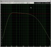
To this end, I will use the SEAS data-sheet frequency plots, and a box simulation made with WinISD.
The Box-volume is 12L, giving a calculated system Q of 0,85 and a Fsc of 75Hz.
The simulation does not take in to account any box-stuffing, so the actual result must be subject to verification through measurement.
The Q of 0,85 gives a slight LF rise, but barely above 0,5 dB, which should be acceptable. This might also be reduced by box stuffing, which could increase the "acoustic volume".
Attachments
Last edited:
The frequency plot on the factory data-sheets are quite detailed, as seems to be customary for SEAS.
The interesting thing will be to see how the drivers behave once they are assembled in to the enclosure. That is what I intend to use as a baseline for any further work.
The interesting thing will be to see how the drivers behave once they are assembled in to the enclosure. That is what I intend to use as a baseline for any further work.
Attachments
The first challenge is therefore to achieve an "anechoic" measurement that will give the response of the drivers plus influence of the boxes.
The gating functionality of the measurement software should do part of the job covering low mid-range and upwards..
Hopefully, the low frequencies can be handled by nearfield measurement.
So, the first challenge will be to see if a nearfield measurement can give a usable LF response, and if this can be combined with a gated farfield measurement to "replicate" an anechoic measurement.
IN the next post I'll post some nearfield measurements and see if that can be of use.
Last edited:
I hope that you will be doing polars of the drivers as well as the completed system. Otherwise just looking at axial data is not going to tell us very much.
Holm is ideal at this task, and I can help with data presentation if you want, but I need the polar data to do that.
Holm is ideal at this task, and I can help with data presentation if you want, but I need the polar data to do that.
Good point!
Well, by polar I assume you mean off-axis plots?
I have obtained a crude but functional turn-table to that end ( The sort you use for Porcelain painting, from my late Grandmother).
But I Thought it was a good idea to sort out the low frequency nearfield measurements first, and then expand with gated farfield measurements both on- and Off-axis.
For the sake of making the thread as "educational" as possible, I'll try to do things one step at a time, getting it right before moving on! 🙂
Very happy to have your comments Dr. Geddes, considering the knowledgeable contribution you have made on numerous other topics, I'm sure your advice can be of great help to guide this thread in a direction that may hopefully make it in to a useful tutorial for those of us doing this for the first time! 🙂
Last edited:
Dr. Geddes,
Despite your advise, I did the low frequency near-field measurements first.
1:
The set up was easy, I just put the mic as close as I could to the woofer cone.
2:
I was curious if it would actually work, it seamed to good (easy) to be true.
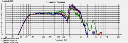
I placed the mic in 3 different positions:
1: As close as possible to centre (next to the phase-plug) (blue)
2: Midway between the phase-plug and the cone-edge (red)
3: Next to the cone edge (green)
The first plot shows the response from the three different positions with the gate function active.
Now, this doesn't quite resemble the original woofer data-sheet plot or the calculated box plot..
At this point I thought that nearfield measurement would not work after all, for no good reason I could identify..
Despite your advise, I did the low frequency near-field measurements first.
1:
The set up was easy, I just put the mic as close as I could to the woofer cone.
2:
I was curious if it would actually work, it seamed to good (easy) to be true.
I placed the mic in 3 different positions:
1: As close as possible to centre (next to the phase-plug) (blue)
2: Midway between the phase-plug and the cone-edge (red)
3: Next to the cone edge (green)
The first plot shows the response from the three different positions with the gate function active.
Now, this doesn't quite resemble the original woofer data-sheet plot or the calculated box plot..
At this point I thought that nearfield measurement would not work after all, for no good reason I could identify..
Attachments

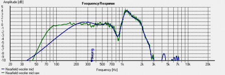
Then it struck me that switching the gating off could improve matters. After all, the purpose of near field measurements is to eliminate room and radiation effects through measuring the immediate pressure variations at the extreme proximity thus eliminating the need for gating in the first place.
The next plot represents the same near field measurements without gating.
Obviously, the response goes a bit haywire above 700 Hz, but that was expected, and according to theory that states that frequencies with wavelength equaling the cone radius (or above) can not be measured nearfield.
The variation in the different measurement positions doesn't seem to be that huge either..
Now the low frequency response seems to correlatew rather well with the calculated response plot!
Attachments
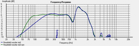
But which of the three measurements positions are best in terms of true representation?
The white paper by D. B. Keele Jr. explains that the ideal is a on axis position, so I'll use that from now on.
The next plot shows the gated and raw measurement superimposed.
The white paper by D. B. Keele Jr. explains that the ideal is a on axis position, so I'll use that from now on.
The next plot shows the gated and raw measurement superimposed.
Attachments
The raw response curve is smooth enough to give a good impression, but I decided to apply a mild 1/5 octave smoothing, just enough to polish off the worst roughness, yet leave a curve detailed enough to reveal any issues.
To me, this response curve looks very nice, no nasty surprises here. If I have actually achieved a response inside +/- 0,5 dB from around 700 hz down to 80 Hz it is actually much better than I could dare hope for! 🙂
The only thing I notice is a small dip around 350 Hz, but considering width and magnitude, I would not think it significant.
Now, this is where I need to ask the following questions:
1:
At which frequency (upwards) does the measurement start to become unreliable? e.g. has the response started to rise or fall before the curve says so?
2: Are there any significant factors concealed by the nearfield measurement that I would have liked to reveal?
3: Did I miss something obvious??
If this measurement turns out to be valid, the next step will be to obtain a good far field measurement and splice it correctly with the near field measurement...
This is where I invite correctives and comments! 🙂
Attachments
Last edited:
Only the green curve is valid, and below 300 Hz it doesn't really matter which position that you use.
Yes, yes of course!
The blue curve with the gated response was only really left in for comparison! 🙂
Do you think I have a good measurement/ result here, or do I need to reiterate something??
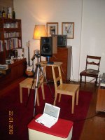
And finally, a picure of my measurement set-up, true DIY! 😀
The blue curve with the gated response was only really left in for comparison! 🙂
Do you think I have a good measurement/ result here, or do I need to reiterate something??
And finally, a picure of my measurement set-up, true DIY! 😀
Attachments
I think the dip and peaking are related (or worsened) to placing the microphone too close to the speaker. Datasheet curves are measured at 53cm.
Yes, yes of course!
The blue curve with the gated response was only really left in for comparison! 🙂
Do you think I have a good measurement/ result here, or do I need to reiterate something??
Looks very typical of what I get - now move on the important stuff.
Hi Elbert,
This looks reasonable for a rough LF curve although quite frankly the TS modeled curve will likely be more accurate than any LF curve you can measure. I've found that a decent outdoor nearfield comes very close to the predicted curve usually for a sealed box. Work on getting an accurate curve above 300 Hz because you can always model the LF curve with good result. Hopefully you have a little more room to measure-hard to tell from the pix exactly.
I agree with Dr. Geddes though, work on measuring the region above 300 and get some off axis curves. I think it will be difficult to optimally use the DXT with a Seas excel since the shallow waveguide doesn't go as low as you'd like from a directivity standpoint. I think you'll still end up with a dip and peak in the power response...
Hi Elbert,
Work on getting an accurate curve above 300 Hz because you can always model the LF curve with good result. .
Modeling the region of small importance (LFs) is easy, but getting the region of critical importance (HFs) is very tough. Don't get lost in all the LF mumbo jumbo. In the end its how the speaker, and the subs of course, work in the actual room that matters, not what the TS or nearfield looks like. Those things don't really matter at all.
I fully agree, something that actually works in the listening room is ultimately the goal here, but I figure a good baseline is beneficial so that I have something to gauge changes against.
From your comments, I understand that getting a far field plot down to 300 Hz is of the essence here.
With the set up and room I have available, I should have about 1m of free space in any direction.
In theory, that should allow me to measure down to 344 Hz.
Having said that, my improvised measurement stand will inevitably give some reflections, so it will be interresting to see what happens and what I can achieve through experimenting with mic-placement and software settings.
Hope I get time to do it this evening! 🙂
One more thing.. considering that I will eventually bring the tweeter in to the picture, should I measure on the woofer axis, the tweeter axis, or somewhere in between??
Last edited:
And with regards to tweeter integration, Looking at what SEAS achieved in their last kit, there should be some hope:
THE ART OF SOUND PERFECTION BY SEAS - Idunn
THE ART OF SOUND PERFECTION BY SEAS - Idunn
One more thing.. considering that I will eventually bring the tweeter in to the picture, should I measure on the woofer axis, the tweeter axis, or somewhere in between??
I would do all the emasurements in the final enclosure with the tweeter in place. I would tend to do it midway between the two drivers, or maybe a little closer to the tweeter. Its not going to be too critical what you choos here unless you are too close.
- Status
- Not open for further replies.
- Home
- Loudspeakers
- Multi-Way
- Measurement approach, 2-way closed box