How exactly does one derive the Laplace transform for some arbitrary equalization curve for use in LTSpice?
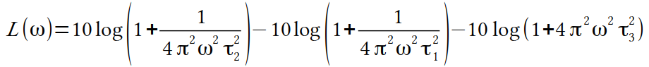
For equalization curves with three inflection points (like RIAA, the Columbia Lp curve, NAB, the London Lp curve) the curve is defined according to the formula in my first attachment. Where ω is the frequency, L(ω) is the gain/loss in decibels at frequency ω, and the τ terms are the time constants for the three inflection points.
Tau 1 is equal to the treble time constant, Tau 2 is equal to the turn-over time constant, and Tau 3 is the bass shelving time constant. For RIAA, these would be 75, 318, and 3180 microseconds respectively. For the Columbia Lp, these would be 100, 318, and 1590 microseconds respectively, and so on...
The form of the Laplace for this curve seems to be:
laplace (1 + Tau 2*s) / (1 + Tau 3*s) / (1+ Tau 1*s)
...and indeed I can get this to work in LTSpice for any curve with three inflection points and match known inverse curves elsewhere.
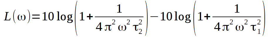
What I can't seem to get to work are curves of the second type, with no shelving time constant and only two inflection points (see my second formula posted). What is the correct form of the Laplace for curves of this second type?
For example, I would like an inverse network for the Columbia 78 curve which has a turn-over time constant of 530 microseconds and a treble time constant of 100 microseconds, and no defined bass-shelving. Any help here would be immensely appreciated; I'm at my wits' end.
Thank you in advance,
Ben
For equalization curves with three inflection points (like RIAA, the Columbia Lp curve, NAB, the London Lp curve) the curve is defined according to the formula in my first attachment. Where ω is the frequency, L(ω) is the gain/loss in decibels at frequency ω, and the τ terms are the time constants for the three inflection points.
Tau 1 is equal to the treble time constant, Tau 2 is equal to the turn-over time constant, and Tau 3 is the bass shelving time constant. For RIAA, these would be 75, 318, and 3180 microseconds respectively. For the Columbia Lp, these would be 100, 318, and 1590 microseconds respectively, and so on...
The form of the Laplace for this curve seems to be:
laplace (1 + Tau 2*s) / (1 + Tau 3*s) / (1+ Tau 1*s)
...and indeed I can get this to work in LTSpice for any curve with three inflection points and match known inverse curves elsewhere.
What I can't seem to get to work are curves of the second type, with no shelving time constant and only two inflection points (see my second formula posted). What is the correct form of the Laplace for curves of this second type?
For example, I would like an inverse network for the Columbia 78 curve which has a turn-over time constant of 530 microseconds and a treble time constant of 100 microseconds, and no defined bass-shelving. Any help here would be immensely appreciated; I'm at my wits' end.
Thank you in advance,
Ben
Attachments
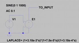
Hopefully this will help:
LAPLACE= (1+3.18e-3*s)*(1+7.5e-5*s)/(1+3.18e-4*s) and see the attachment below.
Edit: I misread your post so this probably isn't helpful, and I no longer exactly remember how to do the transform.
I would have thought it would be only the 2nd (tau 3) and 3rd (tau 1) term in the equation, alternately you could place the bass shelf an order of magnitude lower which ought to work?
Attachments
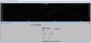
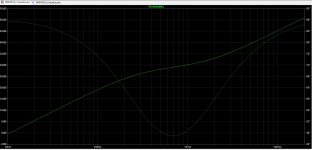
No, that's what I had tried initially as well. The curve would look like this (the playback characteristic). Obviously the recording characteristic would just be the playback characteristic flipped about the x-axis. The limit as frequency heads toward zero looks to be infinity? And the limit as frequency heads toward infinity looks to be heading toward infinity?
Perhaps LTSpice is trying to perform calculations that give division by zero and thus non-nonsensical results? Maybe there isn't a Laplacian that gives just two inflection points?
Perhaps LTSpice is trying to perform calculations that give division by zero and thus non-nonsensical results? Maybe there isn't a Laplacian that gives just two inflection points?
Attachments

The limit as frequency heads toward zero looks to be infinity?
That (ideal) curve has a pole at the origin, so the transfer function would have a factor of 1/s.
At HF, the 100uS pole does take the magnitude toward zero, like the (original) RIAA curve.
Kevin was right, just use a second pole at a very low frequency, around 2Hz-20Hz.
There won't be that much gain available, anyway. As its time constant gets very large
(as pole frequency s0 gets very small), its transfer function factor 1/(s + s0) approaches 1/s.
Last edited:
I think the results are correct for the LaPlace transform I wrote, I think we're missing some fundamental understanding of the transform would be my guess.
Perhaps it is just easier to simulate using RC networks.
Perhaps it is just easier to simulate using RC networks.
Someone posted a reply that has disappeared that solves the problem. There is no circuit that gives infinite gain (which makes sense) thus I should treat this as a circuit with three time constants, and select a bass shelving time constant myself. Now the question becomes, what should I choose for it?
If I select a very, very low frequency, then my calculations for the bass portion of a split passive equalization network become ridiculous to actually implement. Obviously the cutting head(s) that cut my Columbia 78s weren't cutting information at 1 Hz or 2 Hz. But was there meaningful musical information at say, 20 Hz? 30 Hz? 40 Hz?
Perhaps for a 78 a good compromise value would be 30 Hz or 40 Hz?
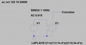
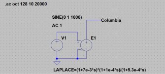
I tried this, and what Rayma said makes sense, so my earlier comment might have been closer to the mark..
LAPLACE=(1+s)*(1+1e-4*s)/(1+5.3e-4*s)
Note: I made a correction and this looks more reasonable. (replaced both attachments and modified the equation)
LAPLACE=(1+s)*(1+1e-4*s)/(1+5.3e-4*s)
Note: I made a correction and this looks more reasonable. (replaced both attachments and modified the equation)
Attachments
<snip>
Perhaps for a 78 a good compromise value would be 30 Hz or 40 Hz?
I would say 30Hz might be a good starting point to roll off the LF boost. I would say add a zero (?) at around 7000us in the simulation and see where that gets you. Shown below..
Attachments

- Status
- Not open for further replies.
- Home
- Design & Build
- Software Tools
- Determining the Laplace Transform for Inverse Equalization Curves in LTSpice?