Mike,
Sorry about your head. Where have I gone wrong?
We have to make a break in the feedback from the output. Let's call the S1 side of the break Vo' to distinguish it from Vo.
Let's call Vn = K1's input voltage
From your fig 1,
Vn = K3.{ Vi - K2.(V'o - Vn) }
Vn = K3.Vi - K3.K2.V'o + K3.K2.Vn
Vn.( 1 - K2.K3 ) = K3.Vi - K2.K3.V'o
for loop gain we want zero input signal, so make Vi=0.
Vn.(1 - K2.K3) = -K2.K3.V'o
Vn/V'o = -K2.K3/(1 - K2.K3)
Vo is equal to Vn.K1,
loop gain = Vo/Vo' = -K1.K2.K3/(1 - K2.K3)
my mistake, shouldn't have added the comma
http://www.control.lth.se/~kja/modeluncertainty.pdf
From K J Astrom “Model Uncertainty and Robust Control”
“fair use” excerpt:
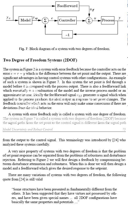
Be sure to read that last para!
http://www.control.lth.se/~kja/modeluncertainty.pdf
From K J Astrom “Model Uncertainty and Robust Control”
“fair use” excerpt:
Be sure to read that last para!
I am begining to wonder whether this is where the mistakes are being made. A non-linear gain block should not be modelled as a linear gain block PLUS an error term. This is mathmatical folly because if you then manipulate your equations as if this "addition" holds true your equations will be wrong. Again, addition and subtraction do not work in a non-linear function (by definition).Hint: K1 is error + ideal output stage gain.
traderbam said:Mike,
Sorry about your head. Where have I gone wrong?
We have to make a break in the feedback from the output. Let's call the S1 side of the break Vo' to distinguish it from Vo.
Let's call Vn = K1's input voltage
From your fig 1,
Vn = K3.{ Vi - K2.(V'o - Vn) }
Vn = K3.Vi - K3.K2.V'o + K3.K2.Vn
Vn.( 1 - K2.K3 ) = K3.Vi - K2.K3.V'o
for loop gain we want zero input signal, so make Vi=0.
Vn.(1 - K2.K3) = -K2.K3.V'o
Vn/V'o = -K2.K3/(1 - K2.K3)
Vo is equal to Vn.K1,
loop gain = Vo/Vo' = -K1.K2.K3/(1 - K2.K3)
http://www.control.lth.se/~kja/nybok/lectures/fourslides2001/lecture9.pdf
http://encon.fke.utm.my/nikd/Dc_dc_converter/Converter/Blockdia.pdf
http://www.columbia.edu/~ag2363/e3410/mult_sys.pdf
traderbam said:Mike,
From your fig 1,
What are you doing with figure 1 ; what is the point of looking at figure 1?
Are you satisfied that figure 3 is equivalent to figure 1?
Then, to find loop-gain from figure 3, simply multiply the gains round the loop. Period.
This is abundantly clear from the links i have given.
Then surely it must be apparent that you are wrong?
Finding out why is down to you.

janneman said:...we have a system that - with the simple tuning of a passive voltage divider - can actually reduce distortion to zero and even go beyond this null and make the distortion re-appear in opposite phase...
Jan Didden
This, consistent with Bob's experience, is what i would expect of an error-cancellation-by-feedback system.
Mike,
No I don't think fig 2 or fig 3 are equivalent to fig 1. Reason: K1 is a non-linear function.
In fig 2 you have assumed that K1.1/K1 = 1.
But K1 is a non-linear function so this does not hold true.
Example: suppose K1(x) = x^3. Therefore 1/K1(x) = 1/(x^3).
K1.1/K1 = (x^3)/[ (x^3)^3 ] = 1/(x^6).
This does not equal x.
To make fig 2 work you need to define the inverse of K(x)...let's call this G(x). You define G(x) such that G[K(x)] = x.
traderbam said:Mike,
No I don't think fig 2 or fig 3 are equivalent to fig 1. Reason: K1 is a non-linear function.
Brian,
This is nonsense.
You are confusing ''non-linear system'' with a distortive linear system.
Clearly K1 is the later, and is not, therefore, a non-linear function.
In fact, K1 is K plus ''disturbance'' or ''error'' as described in the countless links to literature i have given (and you clearly haven't bothered to read!!) and used by Cordell.
So you are modelling a linear function plus error term that is not meant to model a non-linear function. What's the point of that? Good grief!
Don't take my word for it, genius, go simulate your model, with the non-linear terms correctly modelled and you'll see. You'll get the same sort of loop gain result that we get when simulating Bob's output stage. Then you can thank me. 😎
Don't take my word for it, genius, go simulate your model, with the non-linear terms correctly modelled and you'll see. You'll get the same sort of loop gain result that we get when simulating Bob's output stage. Then you can thank me. 😎
traderbam said:You'll get the same sort of loop gain result that we get when simulating Bob's output stage.
Brian,
Actually, the methods used for your simulation for minor loop transmission were in significant error.
More home work for you, old chap. 😎
traderbam said:So you are modelling a linear function plus error term that is not meant to model a non-linear function.
Even more homework:
Find out the definition and true meaning of a ''non-linear'' system, and a nominally linear one with ''disturbance'' (or ''error'') added from the Control literature.
janneman said:
Well, that is where I have my problem in understanding this. On the one hand, we have a system where the distortion reduction cannot ever be complete - the best that can be done is, with infinite loop gain - to assymptotically get closer and closer to zero but never getting there.
On the other hand we have a system that - with the simple tuning of a passive voltage divider - can actually reduce distortion to zero and even go beyond this null and make the distortion re-appear in opposite phase.
I fail to see why these two systems would be fundamentally the same - I would say they are fundamentally different.
Jan Didden
Because we don’t have any such generally nullable system, you keep “forgetting” that at least one (both really for any hardware implementation) of the nulled quantities is a finite bandwidth system so the cancellation can only occur at a finite number of points where the complex frequency response having both phase and amplitude equal intersect
nulling a complete frequency response curve is equivalent to having complete knowledge of the system, in which case a pre-emphasis filter is all that is necessary
Since we are trying to improve an uncertain and externally disturbed system the perfect null is an impossibility – and the systems under discussion are equivalent to 2 degree of freedom feedback with possible loop gain peaks from the finite cancellation null points
jcx said:
maybe they read I. M. Horowitz "Synthesis of Feedback Systems", 1963
7.15 Systems with Combined Positive and Negative Feedback; Zero Senistivity Systems
{1st 2 sentences: }
“ The literature on feedback systems is replete with claims of extraordinary benefits available from systems with minor positive feedback loops. The fallacy in these claims is usually due to lack of consideration of sensitivity (or loop transmission) as a function of frequency.”
{latter: }
"Positive feedback around active elements is a legitimate tool of active network synthesis, and it should be regarded as such and no more. For example if a very small sensitivity at a specific frequency is desired, then positive feedback is a convenient means of realizing a pole of L(jw)" very close to the jw axis…
…However it has never been shown that the gain-bandwidth available from an active device can be increased by positive feedback"
jcx said:I can’t tell if jann and Rodolfo are giving up too soon on trying to understand this feedback fundamental – Rodolfo’s statement seems to still draw a distinction that simply doesn’t exist, the various topologies put forward may result in different implementations depending on the mapping of arithmetic to hardware but they are all equivalent to linear feedback systems with command feedforward, 2-degree of freedom feedback systems with the same stability limits and distortion reducing potential when implemented with similar gain-bandwidth devices – not an interesting coincidence, but a fundamental equivalence
.......
Ok.
What I want to stress is the approach, the strategy, the thought process that leads to formulate a certain design.
In practical terms, it is irrelevant whether, to focus in a particular issue, the summing node of the error correction topology or the driving stage of a cannonical negative feedback configuration ends up being as close to practical to an ideal integrator.
For the cannonical negative feedback, one designs for the maximally achievable open loop gain. As a consequence, dominant pole compensation to ensure stability ends in a high gain low frequency pole. The designer translated the goal to hardware with gain in mind and traded off as little as possible, but as we all know the vast majority of extant operational amplifiers feature this gain-frequency behavior.
For the error correction feedback approach, the designer wants to have an as linear as possible summing node (with the widest possible bandwidth). Since any practical design must acknowledge some form of bandwidth restriction is unavoidable, form the modeling perspective a handy linear model must accept at least one pole somewhere. The net result, this stage when analyzed individually but including the inner positive feedback loop under the error cancelation conditions (unity loop gain), behaves equally as an integrator.
Both approaches, which may rely on totally different hardware implementations, result equivalent. Perhaps this is once more a merry joke Nature is thowing at us as it has happened many times before, underscoring there is something else buried below.
I must remark I find not enlightening at all to insist in a reductionist approach on the lines as here that, being error correction and negative feedback in the end from the realization standpoint equivalent, then one of them should be discarded altoghether. This only precludes alternative points of view, and science has made progress only through disparate ramblings and alternative perspectives, subject later of course to the merciless reality check.
A note to happy block diagrammers, I have no objections for those who prefer to juggle block diagrams instead of boring algebra, but to happily insert a time-reversing cause-reversing block makes me shudder. I do not like diagrams that cannot realte directly to hardware but then it may be my own personal limitation.
Rodolfo
ingrast said:A note to happy block diagrammers, I have no objections for those who prefer to juggle block diagrams instead of boring algebra, but to happily insert a time-reversing cause-reversing block makes me shudder. Rodolfo
Where?
You cannot have ''time-reversing'' in a time-invariant system.
jcx said:
Because we don’t have any such generally nullable system, you keep “forgetting” that at least one (both really for any hardware implementation) of the nulled quantities is a finite bandwidth system so the cancellation can only occur at a finite number of points where the complex frequency response having both phase and amplitude equal intersect
This, i would suggest, is all we're interested in: error cancellation in the audio band, and nothing but.
I fail to see how such a modest NFB system may possess significant singularities in the audio band.
The fact that phase relationships stray (as they invariably do with any NFB system) from the desired optimum for error cancellation at HF then becomes irrelevant.
Be that as it may, it is to be expected that practical implementations of this stratagem are inevitably compromised by non-linearity in the summers, which is accommodated in the user-adjustable blocks here.
The later, as noted by Bob in his paper, will take the form of a potentiometer at one or other summing junctions.
Re: Final contribution
Thank you for your participation. I think I agree with everything you have said.
Bob
ingrast said:Gentlemen,
I should like to wrap up my involvement for the time being with a summary.
Error correction represents an error reducing design strategy different from conventional negative feedback. This holds no matter the fact actual realization happens to translate into equivalent formal gain expresions.
I want to emphasize the "design strategy" concept, for by topology, the objective is to null error by comparing plant input and output.
- Implicitely, as a consequence of implementation with real elements the correction factor increases with decreasing frequency reaching a theoretical infinite at DC.
Interestingly, negative feedback systems with extremely high open loop gain usually insert a very low frequency dominant pole, yielding a similar correction/attenuation performance.
- Stability is an issue but then it is also an issue in conventional negative feedback systems where open loop gain is very high.
- Implementation is straightforward with the current generation of available devices.
Rodolfo
Thank you for your participation. I think I agree with everything you have said.
Bob
mikeks said:
Where?
.....
The 1/K1 block. Please take your time and think carefully before firing from the waist.
Rodolfo
- Home
- Amplifiers
- Solid State
- Bob Cordell Interview: Error Correction