I hope this is not off topic. Excuse me if I'm wrong.
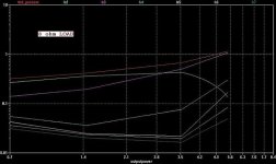
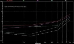
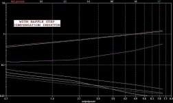
I simulated three variants. My SET amplifiers loaded with 8 ohm resistor, loaded with XO+Speaker (without baffle step compensation inductor) and XO+Speaker with baffle step compensation. All depending on output power of the amplifier.
Behavior of harmonics from H2 to H5 are very interesting, in any case.
PLEASE do not open a discussion about crossover or so. I just want to show the possibilities of this THD analyzer as I see it.
Thank you all.
Attachments
I created an LTSPICE add-on to automate THD measurements and plot result in the form of THD vs. Amplitude and THD vs. Frequency graphs.
I was inspired by "jfet_amp_disto_plot" by Helmut Sennewald, "Audio Distortion Analyser" by Tony Casey and "Fundamental Null Distortion Residual" by jcx from http://www.diyaudio.com/forums/software-tools/101810-spice-simulation-37.html#post133313
THD_Analyzer.zip contains all necessary files and example. Unzip all files in the same directory, open “Example_BJT_THD_TEST.asc” and run simulation.
You can monitor analysis progress in the left lower corner of LTSPICE window. After simulation and analysis is complete (including completion of .MEASURE), follow the instructions to display
results.
Very

-RNM
Very nice looking graphs!
What I'd like to do is state a number for THD ( percent of each harmonic would be excellent). Could you please explain a lilttle about the contents of the output error log file? What do the variables ah1c, ah2s etc mean? It looks like they make up my answer somehow....
THANK YOU FOR THIS!!!
What I'd like to do is state a number for THD ( percent of each harmonic would be excellent). Could you please explain a lilttle about the contents of the output error log file? What do the variables ah1c, ah2s etc mean? It looks like they make up my answer somehow....
THANK YOU FOR THIS!!!
I have used this very handy little tool many times with no troubles some time ago and haven't used it more recently for a while, and now that I am trying to use it again, I'm getting an error that I can't make any sense of.
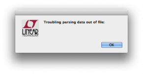
The measurement that I was trying to do was done with a fair amount of resolution, so although I am running on a machine with 8 cores, it took more than 10 hours to run through, but after all that time running, monopolising most of the processor and grabing close to 40gb of disk space, when I tried getting the plot done from the log, I got this error as shown in the attached screen shot.
I guess this means the whole thing was just a huge waste of time and will have to be done again, but with the risk of getting this same error again.
What could be the cause of this? How can I prevent this from happening?
Any ideas?
Attachments
I've never seen this message. I'm expecting that this was happening because amount of data was very big. Though, I don't know for sure.
This tool produce a lot of data and is time consuming. It happens because it makes multiple runs of transient analysis. One run per every point of frequency or amplitude. Try to reduce amount of steps in amplitude or frequency.
This tool produce a lot of data and is time consuming. It happens because it makes multiple runs of transient analysis. One run per every point of frequency or amplitude. Try to reduce amount of steps in amplitude or frequency.
I've never seen this message.
Perhaps this never happened on windoze, and it's a bug on mac osx.
You're probably right. I've never seen this until now, and I did notice that humongous data file, almost 40gb. I wanted a higher resolution, so the simulation ran for more than 10 hours, and dumped that mega sized file as a result.I'm expecting that this was happening because amount of data was very big. Though, I don't know for sure.
Maybe there is a bug that rears its uggly head when there is too much data.
My machine has plenty of ram (32gb), and far more than enough free drive space (over 600gb), so nothing was maxed out, by a long shot. Not even the processors, that never really were fully utilized (8 cores). So the bug option may just be the only one...
No kidding! And if we want better resolution, yikes!This tool produce a lot of data and is time consuming. It happens because it makes multiple runs of transient analysis. One run per every point of frequency or amplitude.
I'll have to try that. I was just trying other simulations from before that ran with no issues, and they still run now. I'm trying progressively with higher resolutions, to see if I run into this again. Then I'll try again the one that failed...Try to reduce amount of steps in amplitude or frequency.
Thanks a lot for that super tool! Very nice!
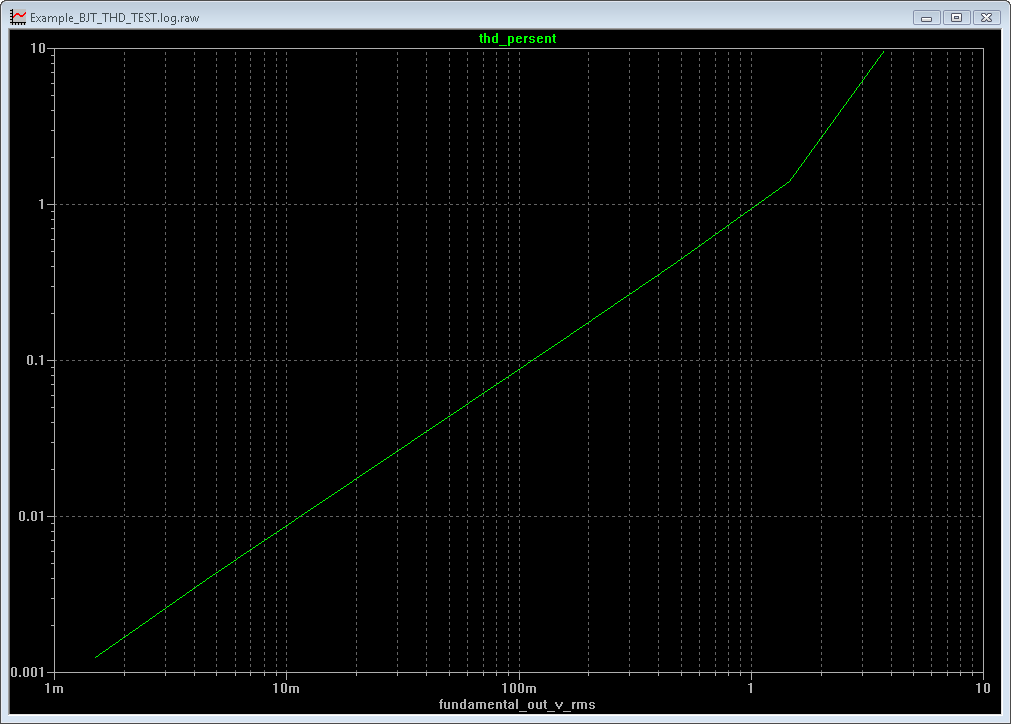
One more question: I didn't remember having seen the thd_percent curve with a vertical scale with the numbers having an "m".
I'm guessing this means something like "milli" despite the fact that percent has no real unit (except the % sign), and that the 270m for example just means 0.27%
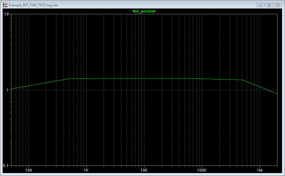
This was done on a power amp. I'm just trying to see how the distortion is at each end of the band. Why not just stay in % ?
I'm guessing this means something like "milli" despite the fact that percent has no real unit (except the % sign), and that the 270m for example just means 0.27%
This was done on a power amp. I'm just trying to see how the distortion is at each end of the band. Why not just stay in % ?
Attachments
Hello Eugene,
first of all thanks for this wonderful tool!
I'm sorry to resurrect this somehow old topic, nevertheless it seems the log file report some errors and warnings, even if it seems to work ok (I can plot the curves and the obtained values seems in agreement with the ones I can retrieve usinf the LTSpice fft directive):
Code:
Circuit: * D:\Elettronica\LTSpice_Librerie\THD_Analyzer\Example_BJT_THD_TEST.asc

Questionable use of curly braces in "b_time timescale 0 v={time}"
    Error: undefined symbol in: "[time]"
WARNING: Less than two connections to node TIMESCALE.  This node is used by B:U2:_TIME.
WARNING: Less than two connections to node S_TIME.  This node is used by B:U2:_STROBETIME.
WARNING: Less than two connections to node E_TIME.  This node is used by B:U2:_ENDTIME.
WARNING: Less than two connections to node H2SF.  This node is used by B:U2:_H2S.
WARNING: Less than two connections to node H2CF.  This node is used by B:U2:_H2C.
WARNING: Less than two connections to node H3SF.  This node is used by B:U2:_H3S.
WARNING: Less than two connections to node H3CF.  This node is used by B:U2:_H3C.
WARNING: Less than two connections to node H4SF.  This node is used by B:U2:_H4S.
WARNING: Less than two connections to node H4CF.  This node is used by B:U2:_H4C.
WARNING: Less than two connections to node H5SF.  This node is used by B:U2:_H5S.
WARNING: Less than two connections to node H5CF.  This node is used by B:U2:_H5C.
WARNING: Less than two connections to node H6SF.  This node is used by B:U2:_H6S.
WARNING: Less than two connections to node H6CF.  This node is used by B:U2:_H6C.
WARNING: Less than two connections to node H7SF.  This node is used by B:U2:_H7S.
WARNING: Less than two connections to node H7CF.  This node is used by B:U2:_H7C.
WARNING: Less than two connections to node H8SF.  This node is used by B:U2:_H8S.
WARNING: Less than two connections to node H8CF.  This node is used by B:U2:_H8C.
WARNING: Less than two connections to node H9SF.  This node is used by B:U2:_H9S.
WARNING: Less than two connections to node H9CF.  This node is used by B:U2:_H9C.
WARNING: Less than two connections to node H10SF.  This node is used by B:U2:_H10S.
WARNING: Less than two connections to node H10CF.  This node is used by B:U2:_H10C.
Direct Newton iteration for .op point succeeded.
Ignoring empty pin current: Ix(u2:analyzer_in)
Ignoring empty pin current: Ix(u2:analyzer_in)
.step ag=0.001
.step ag=0.00215443
.step ag=0.00464159
.step ag=0.01


Measurement: ah1s
  step	v(ref_s)	at
     1	-0.0103440360141	0.01
     2	-0.0222856572219	0.01
     3	-0.0480127157217	0.01
     4	-0.103436042359	0.01

Measurement: ah1c
  step	v(ref_c)	at
     1	-0.000651384162325	0.01
     2	-0.0011994512681	0.01
     3	-0.00238019358308	0.01
     4	-0.00492370764634	0.01

Measurement: avh2s
  step	v(h2sf)	at
     1	-1.63234541406e-007	0.02
     2	-7.09703741115e-007	0.02
     3	-3.19213504035e-006	0.02
     4	-1.46046463495e-005	0.02

Measurement: avh2c
  step	v(h2cf)	at
     1	1.32446413721e-006	0.02
     2	6.14886066862e-006	0.02
     3	2.85409337516e-005	0.02
     4	0.000132539670176	0.02

Measurement: avh3s
  step	v(h3sf)	at
     1	-1.45688078842e-008	0.02
     2	-4.46070611872e-008	0.02
     3	-2.28286942682e-007	0.02
     4	-1.80868618291e-006	0.02

Measurement: avh3c
  step	v(h3cf)	at
     1	-7.10073891694e-010	0.02
     2	-2.13512336777e-009	0.02
     3	-2.291879299e-008	0.02
     4	-2.4236855999e-007	0.02

Measurement: avh4s
  step	v(h4sf)	at
     1	-9.67061183294e-009	0.02
     2	-2.09281986124e-008	0.02
     3	-4.58763103106e-008	0.02
     4	-1.00083024035e-007	0.02

Measurement: avh4c
  step	v(h4cf)	at
     1	-6.60220682057e-010	0.02
     2	-1.58822150389e-010	0.02
     3	-4.41697924212e-010	0.02
     4	-2.20961747671e-008	0.02

Measurement: avh5s
  step	v(h5sf)	at
     1	-7.73415191509e-009	0.02
     2	-1.67464142265e-008	0.02
     3	-3.68403735269e-008	0.02
     4	-8.30140989326e-008	0.02

Measurement: avh5c
  step	v(h5cf)	at
     1	-7.46715946549e-010	0.02
     2	-3.03754773743e-010	0.02
     3	1.56623364977e-010	0.02
     4	-1.08824711186e-009	0.02

Measurement: avh6s
  step	v(h6sf)	at
     1	-6.44263507967e-009	0.02
     2	-1.39529655565e-008	0.02
     3	-3.07022927487e-008	0.02
     4	-6.94114636535e-008	0.02

Measurement: avh6c
  step	v(h6cf)	at
     1	-7.95309867629e-010	0.02
     2	-4.08114221247e-010	0.02
     3	-7.10896553215e-011	0.02
     4	-1.64330318833e-009	0.02

Measurement: avh7s
  step	v(h7sf)	at
     1	-5.51981240886e-009	0.02
     2	-1.19579870626e-008	0.02
     3	-2.63144476704e-008	0.02
     4	-5.9486448132e-008	0.02

Measurement: avh7c
  step	v(h7cf)	at
     1	-8.24502695445e-010	0.02
     2	-4.70795468538e-010	0.02
     3	-2.07098648287e-010	0.02
     4	-1.94438930101e-009	0.02

Measurement: avh8s
  step	v(h8sf)	at
     1	-4.8278263026e-009	0.02
     2	-1.04612540499e-008	0.02
     3	-2.30230527465e-008	0.02
     4	-5.20430903953e-008	0.02

Measurement: avh8c
  step	v(h8cf)	at
     1	-8.43322181187e-010	0.02
     2	-5.11953070526e-010	0.02
     3	-2.95177784282e-010	0.02
     4	-2.1369284653e-009	0.02

Measurement: avh9s
  step	v(h9sf)	at
     1	-4.28874103126e-009	0.02
     2	-9.29735086578e-009	0.02
     3	-2.04634736647e-008	0.02
     4	-4.62536712994e-008	0.02

Measurement: avh9c
  step	v(h9cf)	at
     1	-8.56351020488e-010	0.02
     2	-5.3993012188e-010	0.02
     3	-3.56000619236e-010	0.02
     4	-2.26850194833e-009	0.02

Measurement: avh10s
  step	v(h10sf)	at
     1	-3.85801491992e-009	0.02
     2	-8.36581824371e-009	0.02
     3	-1.84156139533e-008	0.02
     4	-4.16210659899e-008	0.02

Measurement: avh10c
  step	v(h10cf)	at
     1	-8.65660748775e-010	0.02
     2	-5.59766992165e-010	0.02
     3	-3.99415703031e-010	0.02
     4	-2.36277309079e-009	0.02

Measurement: i_in_s
  step	v(is_s)	at
     1	-4.8186020519e-008	0.01
     2	-1.03813614681e-007	0.01
     3	-2.23659423724e-007	0.01
     4	-4.81857145954e-007	0.01

Measurement: i_in_c
  step	v(is_c)	at
     1	-1.0711486489e-009	0.01
     2	-2.30771654808e-009	0.01
     3	-4.97179587315e-009	0.01
     4	-1.07111372461e-008	0.01

Measurement: fundamental_out_v_rms
  step	sqrt(2)*hypot(ah1s,ah1c)
     1	0.0146576520895
     2	0.0315622939963
     3	0.0679836185042
     4	0.146446288829

Measurement: fundamental_out_dbu
  step	20*log10(fundamental_out_v_rms/0.774596669)
     1	-34.4602243177
     2	-27.7981412836
     3	-21.1334269677
     4	-14.4679450916

Measurement: gain
  step	sqrt(2)*fundamental_out_v_rms/ag
     1	20.7290503775
     2	20.7181143321
     3	20.7134579891
     4	20.7106327822

Measurement: gain_db
  step	20*log10(gain)
     1	26.33158814
     2	26.3270045075
     3	26.3250521568
     4	26.3238673662

Measurement: phase_deg
  step	atan(ah1c/ah1s)
     1	3.60326934866
     2	3.08078200436
     3	2.83807092527
     4	2.72530613667

Measurement: z_in_mod
  step	0.5*ag/(hypot(i_in_s,i_in_c))
     1	10373.8906697
     2	10373.8926245
     3	10373.9032725
     4	10373.9566665

Measurement: z_in_ph_deg
  step	(-1)*atan(i_in_c/i_in_s)
     1	-1.27344383582
     2	-1.27344227699
     3	-1.2734362288
     4	-1.27341041143

Measurement: h2
  step	sqrt(2)*hypot(avh2s,avh2c)*100/fundamental_out_v_rms
     1	0.0128755073885
     2	0.0277341458465
     3	0.0597418086914
     4	0.12876660244

Measurement: h3
  step	sqrt(2)*hypot(avh3s,avh3c)*100/fundamental_out_v_rms
     1	0.0001407310187
     2	0.000200099949835
     3	0.000477275876064
     4	0.0017622377377

Measurement: h4
  step	sqrt(2)*hypot(avh4s,avh4c)*100/fundamental_out_v_rms
     1	9.35221089566e-005
     2	9.377580277e-005
     3	9.54375608219e-005
     4	9.897639001e-005

Measurement: h5
  step	sqrt(2)*hypot(avh5s,avh5c)*100/fundamental_out_v_rms
     1	7.496836642e-005
     2	7.5048099219e-005
     3	7.66370309048e-005
     4	8.0172568859e-005

Measurement: h6
  step	sqrt(2)*hypot(avh6s,avh6c)*100/fundamental_out_v_rms
     1	6.26322750045e-005
     2	6.25458722695e-005
     3	6.3867908401e-005
     4	6.70485678577e-005

Measurement: h7
  step	sqrt(2)*hypot(avh7s,avh7c)*100/fundamental_out_v_rms
     1	5.38476313027e-005
     2	5.36217331114e-005
     3	5.47417188058e-005
     4	5.74760005438e-005

Measurement: h8
  step	sqrt(2)*hypot(avh8s,avh8c)*100/fundamental_out_v_rms
     1	4.72856045342e-005
     2	4.69298986833e-005
     3	4.78971111986e-005
     4	5.02997126282e-005

Measurement: h9
  step	sqrt(2)*hypot(avh9s,avh9c)*100/fundamental_out_v_rms
     1	4.21958648922e-005
     2	4.17288832833e-005
     3	4.25751109166e-005
     4	4.47202820732e-005

Measurement: h10
  step	sqrt(2)*hypot(avh10s,avh10c)*100/fundamental_out_v_rms
     1	3.81487883262e-005
     2	3.75685889826e-005
     3	3.83176660368e-005
     4	4.0257657253e-005

Measurement: thd_persent
  step	sqrt(h2*h2+h3*h3+h4*h4+h5*h5+h6*h6+h7*h7+h8*h8+h9*h9+h10*h10)
     1	0.0128773116951
     2	0.0277353466596
     3	0.0597439463906
     4	0.128778777597

Measurement: thd_db
  step	20*log10(thd_persent/100)
     1	-77.8034958418
     2	-71.1393280315
     3	-64.4741218686
     4	-57.8031140333


Date: Mon Jan 30 14:36:23 2017
Total elapsed time: 15.804 seconds.

tnom = 27
temp = 27
method = modified trap
totiter = 175119
traniter = 175112
tranpoints = 75037
accept = 75033
rejected = 4
matrix size = 75
fillins = 0
solver = Normal
Thread vector: 13.0/7.7[2] 0.8/1.0[1] 5.0/2.9[2] 0.1/0.8[1]  2592/500
Matrix Compiler1: 2.12 KB object code size  1.1/0.5/[0.4]
Matrix Compiler2: 3.85 KB object code size 0.7/0.8/[0.4]How to plot the thd % and on the other axe the Vout(rms) ?
solved
just change X axis from ag to Fundamental_Out_V_RMS
Hi,Eugene,I created an LTSPICE add-on to automate THD measurements and plot result in the form of THD vs. Amplitude and THD vs. Frequency graphs.
I was inspired by "jfet_amp_disto_plot" by Helmut Sennewald, "Audio Distortion Analyser" by Tony Casey and "Fundamental Null Distortion Residual" by jcx from http://www.diyaudio.com/forums/software-tools/101810-spice-simulation-37.html#post133313
How it works:
It outputs sinusoidal signal with amplitude or frequency stepping sweep into device under test (DUT). Output signal from DUT is feed into analyzer input. After waiting some time for signal to become steady state, analyzer restores fundamental and subtracts it from input signal. This subtraction allows to increase resolution or reduce measurement time for the same resolution. You can monitor residual components at “Notch output”.
Residual signal is then fed into synchronous filters and detector. Each harmonic is filtered and measured separately. Maximum of 10 harmonics are analyzed. Amount of harmonics could be easily increased by adding corresponding filters and possessing.
How to use LTSPICE Audio THD Analyzer:
Place THD_Analyzer.asy symbol and Analyser_Controls.txt files in the same directory, where you are saving schematic (DUT schematic),
that you would like to analyze.
Put SPICE directives “.inc Analyzer_Controls.txt” and “.tran 0 {AnalysisTime} {SettlingTime} {MaxTimestep}” in DUT schematic .
Edit “Analyzer_Controls.txt“ to enable (uncomment) appropriate sweep (amplitude or frequency ) and save this file.
Setup “.param Ag=xxx” as amplitude for frequency sweep or “.param Fg=xxx” as frequency for amplitude sweep.
Run the simulation.
After simulation is complete, go to View menu and open SPICE Error Log or use Ctrl+L command.
Click with right mouse button on opened Log file.
Execute “Plot .step’ed .meas data” command. Right mouse button click on opened plot and use Add Trace or Ctrl+A and select the data that you want to plot.
You may want to double click on axis to change axis limits or switch to logarithmic scale.
Notch output shows residual components, after fundamental removal.
Please note that fundamental may not be removed completely. This is not necessarily affecting resolution of measurements as soon as additional synchronous filtering is used to measure amplitude of harmonics.
Increasing SettlingTime and StrobeLength, or (and) decreasing MaxTimestep would likely improve fundamental rejection.
Generator output is DC coupled and has 0 Ohm output impedance. Use external AC coupling and appropriate series resistor if required, to ensure proper operation of simulated circuit.
THD_Analyzer.zip contains all necessary files and example. Unzip all files in the same directory, open “Example_BJT_THD_TEST.asc” and run simulation.
You can monitor analysis progress in the left lower corner of LTSPICE window. After simulation and analysis is complete (including completion of .MEASURE), follow the instructions to display
results.
First of all. Thanks you very much for your wonderful tool.
I have confronted some problems. Could you give me some advice?
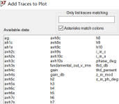
1. I cannot plot the THD vs freq graph.
You said "Double click on horizontal axis label of your distortion plot.
Put fg label name instead of Fundamental_Out_V_RMS".
But the fg cannot be found available data. Please see the attachment.
How to fix this problem.
2.A question of Analyzer_Controls.txt.
In this txt, 2 harmonic, 3 harmonic, 4 harmonic, 5 harmonic, 6 harmonic, 7 harmonic, 8 harmonic, 9 harmonic and 10 harmonic refer to (2*pi*time*Fg), (4*pi*time*Fg), (6*pi*time*Fg), (8*pi*time*Fg), (10*pi*time*Fg), (12*pi*time*Fg), (14*pi*time*Fg), (16*pi*time*Fg), (18*pi*time*Fg) and (2*pi*time*Fg).
The amplifier produces predictable significant amounts of even order THD (the ‘good’ kind) to introduce a warmth to digital recordings. So that many people focus the odd order THD.
My question is whether the Analyzer_Controls.txt only include the even order THD?
Thanks!
Attachments
Hi Eugene,
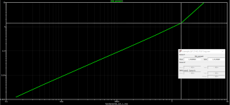
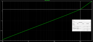
Acoording to your wonderful tool, I can plot the curves of thd_persent vs fundamental_out_v_rms and thd_persent vs ag.
My questions are those.
1. How to understood the meaning of the X-axis and Y-axis of those curves?
2. What is the representation of the line charts? Those are not straight lines.
Thanks!
Attachments
- Home
- Design & Build
- Software Tools
- LTSPICE THD Analyzer