john curl said:Right you are, SY! He overdid it, without realizing what it would do to many amplifiers.
Does it mean that he didn't measured impedance of his loudspeaker project or he didn't realized that amplifiers weren't designed for such low impedance?
At the time that version of the Watt was current the He-man amplifier goal was to drive the Apogee ribbon (.5 Ohm through the whole midrange). Many amps were promoted as able to deliver full power into what was essentially a shorted cable. I thought that was silly since the speaker was such a small part of the market and the additional stuff required did nothing for the sound otherwise (except compromise it). Dave was still pretty unsophisticated in his crossovers at the time. They improved at substantial upgrade costs to his customers (the downside of potted crossovers). Probably not a good fit for a single ended triode amp unless you like that "more distant" sound from the depressed upper midrange.
john curl said:The WATT 1 loudspeaker was published in 'Stereophile' Feb 1988 pp. 88-96. The measured impedance curve is on p. 92. I was wrong, it is 0.33 ohms not 0.5 ohms at 2KHz.
Once again, why? What did Dave Wilson add to the x-over that made this happen?
I have measured it independently, myself.
Thanks, John.
That low impedance is really remarkable. It's hard to imagine what Dave did to get that. Even a deliberate straight series-resonant circuit across the speaker terminals would have to use a pretty good inductor with quite low ESR to get that.
Of course, I'm assuming that the impedance dip is resonant-like rather than over a fairly broad interval. If it is, one has to wonder about the energy storage associated with that resonance.
Even an amplifier with a damping factor of 100 in the 2 kHz region (Zout ~ 0.08 ohms) would seem to suffer nearly 2 dB of frequency response coloration as a result of that.
Also, if I did my math right, a 5 uH output coil in a power amplifier would have an impedance of about 0.063 ohms at 2 kHz, so a frequency response coloration would result from that inductance even if the amplifier had a damping factor ahead of the coil of 1000. This would be an example of where an output coil as large as 5 uH (which most of us agree is too much) would cause an audible difference based on frequency response coloration alone.
All of this is one reason why I wish people (especially those doing reviews) would check the frequency response of the amplifier/loudspeaker combination AT THE LOUDSPEAKER TERMINALS, just to rule out the possibility that differences they are hearing are just ordinary frequency response colorations due to amplifier (+cable) impedance loaded by the speaker impedance.
At least this is an example of a test that can be carried out easily in-situ with a real loudspeaker as a load.
Cheers,
Bob
I have not seen such a spectra.
My numbers were taken from Vogel's book "sound of silence".
NB The unit is dBA and for 33 1/3 LPs. With 45 rpm Vogel writes that -73.5 dBA is possible.
Sigurd
My numbers were taken from Vogel's book "sound of silence".
NB The unit is dBA and for 33 1/3 LPs. With 45 rpm Vogel writes that -73.5 dBA is possible.
Sigurd
scott wurcer said:
If you examine the spectra real time, the actual noise floor is lower than you think. The RMS sum of the impairments give an overly pessimistic number. I have many LP's where the the noise drops noticably between cuts (tape noise is worse).
I use Grado exclusively (400 Ohms) so this is just a fun exercise for me.
Bob Cordell said:
All of this is one reason why I wish people (especially those doing reviews) would check the frequency response of the amplifier/loudspeaker combination AT THE LOUDSPEAKER TERMINALS, just to rule out the possibility that differences they are hearing are just ordinary frequency response colorations due to amplifier (+cable) impedance loaded by the speaker impedance.
At least this is an example of a test that can be carried out easily in-situ with a real loudspeaker as a load.
Cheers,
Bob
That really is good idea, and could be very useful.
Problem is that most of the reviewers can't tell resistor from transistor and measureing anything is just beyond them. I know, I was audio magazine editor in chief

john curl said:
I made two mistakes in the original design that is more than 25 years old now. One important one was where I fed back the servo output back to the input.
I did the same mistake, originally. Fortunately, today we have simulators and the stray noise injection was obvious from the very beginning, even with using a relatively low noise opamp in the servo. That's why the HPS 3.0 servo is wrapped only around the gain stages, avoiding the low noise input stage. Also fortunately, we have today low noise and low offset opamps, so the low noise input stage offset is not impacting the overall headroom.
The WATT 1 still sounds good to me, but I cheat. I put an (older) Bybee device in series with the input in order to add an extra .3 ohm to the load. Works for me, and I get the Bybee to do its thing as well. Besides, the power amp that I am using is rated at 90A peak current output.
When I drive a WATT 1 with a tube amp, it seems to ignore the suck out, probably because it is such a narrow range of frequency.
When I drive a WATT 1 with a tube amp, it seems to ignore the suck out, probably because it is such a narrow range of frequency.
We had SPICE noise simulators 10 years BEFORE I designed the Vendetta in the first place.The only problem is that you had to attend the university at the time. Of course, I hope that you, SYN08, has the IC op amp module for your Quantech, so you can catch things, like out of typical spec IC's from some manufacturers. It is really a QC problem, rather than a design problem, because you can't easily hear random noise below 100 Hz, anyway. That's why they invented the 'A' or the CCIR curves.
scott wurcer said:
Not FET's in particular, physicists like to speak of equal power per freqency band normalized to a one Hz band i.e. volts squared per Hz. To make that plain volts it becomes volts/rt-Hz. For equal bins in an FFT or constant IF BW on a spectrum analyser you get a flat spectrum (white noise).
john curl said:Noise adds up as the square root of sum of the individual noise units squared. This is where the square root comes from.
Ok, I think I get this now. It's like with total harmonic distortion where you sum the squared amplitudes of all the harmonics, and take the square root.
Except with noise you're just normalizing the sum to a one Hz band, that's the way physicists like it? Well, I'm still chewying on this one a bit.
And noise and distortion just add up like that?
Thanks.

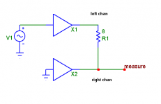
PMA said:I use this method to force output.
Practical, but there is some danger of measuring
crosstalk instead of the residual.
But you surely have yet another amp...
Using a square wave should show how fast
and how good the amplifier corrects output errors.
regards, Gerhard
PMA said:Bob,
I use this method to force output.
Regards,
Pavel
Exactly, same here. A stereo amplifier makes this convenient. There are some tests, however, where the forcing amplifier may want to be a bigger amplifier just to make sure that it is not close to current limiting or under duress in some other way.
Cheers,
Bob
gerhard said:
Practical, but there is some danger of measuring
crosstalk instead of the residual.
But you surely have yet another amp...
Using a square wave should show how fast
and how good the amplifier corrects output errors.
regards, Gerhard
The back-driving technique is also useful for exposing crossover distortion in a more sensitive way. Take the output of the amplifier under test while being back-driven, amplifiy it if necessary, and put it into a THD analyzer (or a spectrum analyzer). The amplifier under test has already done most of the work of getting rid of the fundamental.
In the same way, one can back-drive a 19+20 kHz CCIF two tone signal into the amplifier under test.
Finally, if you want a real LF torture test that will exercise the SOA space of the output stage, drive the amplifier with 19 Hz in the forward path and with 20 Hz in the back-drive path. You will get a 1 Hz envelope total current signal, where the voltage and current of the output stage are run through their various combinations as the 19Hz signal walks past the 20 Hz signal in time. Of course, this also brutally causes the rail current in the amplifier to go from min to max in accordance with the 1 Hz beat frequency. During this test, one can look for any 1 Hz signal at the output of the AUT. One can of course also look for other combinations of 19 Hz and 20 Hz at the output of the AUT with a spectrum analyzer, just like with the CCIF test.
One can go a step further and put a SMPTE IM 60 Hz & 7kHz signal into the forward path of the amplifier under test and back-feed a 59 Hz signal into the amplifier. One can then look for 1 Hz, 59 Hz, 60 Hz and other modulation artifacts on the 7 kHz carrier.
Cheers,
Bob
The 1 Hz bandwidth should not bother you. It is easy to average over a much larger bandwidth by multiplying over the square root of the larger bandwidth.
For example, a 10,000Hz bandwidth looks like 100 times more noise than a 1 Hz bandwidth. IF everything is normalized to 1 Hz, it is easy to do piecemeal approximations, because the noise may be worse at the end of the bands, and have to be totaled separately to get an accurate evaluation of what you are going to get just from the data sheet.
For example, a 10,000Hz bandwidth looks like 100 times more noise than a 1 Hz bandwidth. IF everything is normalized to 1 Hz, it is easy to do piecemeal approximations, because the noise may be worse at the end of the bands, and have to be totaled separately to get an accurate evaluation of what you are going to get just from the data sheet.
- Status
- Not open for further replies.
- Home
- Amplifiers
- Solid State
- John Curl's Blowtorch preamplifier