...
Everything above 200Hz follows a similar pattern I've seen while using REW and UMIC 1 mic. i.e. more SPL on bass and gentle slope down towards 20kHz.
Looks like HF reflections are killing a better FR. BUT no serious lobing effects, which I noticed did disappear for myself after 'curving' both arrays at listening distance 3'-4' away. ...
Excuse me Sir, but I see nothing but serious lobing effects above 1,4kHz, most severe around 3kHz which is a very sensitive area for hearing timbre and localization of sound. JL's graphics show this very well. Naturally, in a room with six boundaries these get more and more mixed.
Obviously a curved tower or delay can alleviate this lobing in vertical plane, but only in a narrow passband related to degree of curvature/delay versus wavelength.
ps. was that "no" missing a t?
Last edited:
Excuse me Sir, but I see nothing but serious lobing effects above 1,4kHz, most severe around 3kHz which is a very sensitive area for hearing timbre and localization of sound. JL's graphics show this very well. Naturally, in a room with six boundaries these get more and more mixed.
Obviously a curved tower or delay can alleviate this lobing in vertical plane, but only in a narrow passband related to degree of curvature/delay versus wavelength.
ps. was that "no" missing a t?
First, let me say I was not notified there was a new post on this thread, hence the long wait for my response. I apologize!
Second, I saw your 4-way active dipole project over at miniDSP. Very cool fellow miniDSP user.
Third, the "no" was not missing a "t"
Fourth, I've got all sorts of reflections, a great many actually and the system sounds very good. Not perfect mind you. Every once in awhile I'll hear a combination of instruments/voices at a certain frequency ~7kHz and I'm like 'ouch'. But for the most part it is a wall of sound that sounds exceptional even without 'simple' EQ using a DEQ2496. No FIR or IIR either, but I'll possibly be looking into that at a later date for experimentation and to expand my knowledge. I've been into DSP since the old days of very expensive 16-bit sample/hold ADC's. Very nice to see the progress we've made!
Cheers!
Last edited:
POST #10
C. Infinite Line Source: frequency-domain pressure response (continued)
Mathematicians are a funny lot. Often, when closed-form solutions to integrals are nowhere to be found ... the integrals are simply "named" in honor of those who wrestle with them. In other words, if a problem can't be 'solved', it simply gets 'named' instead") (yes, i'm being a bit facetious ... but i couldn't resist)
(yes, i'm being a bit facetious ... but i couldn't resist)
Our line source transfer function is a sum of 2 integrals :
H(k) = (rho/2pi)*{INT[cos[kr*cosh[v]]]dv - j*INT[sin[kr*cosh[v]]]dv}, from v=0 to +infinity
The second integral is actually in the form of a rather famous one :
INT[sin[kr*cosh[v]]]dv (from v=0 to +infinity) = (pi/2)*Jo[kr]
where Jo[x] is known as a "zero-order Bessel Function of the 1st Kind"
The first integral is also in the form of a rather famous one :
INT[cos[kr*cosh[v]]]dv (from v=0 to +infinity) = (-pi/2)*Yo[kr]
where Yo[x] is known as a "zero-order Bessel Function of the 2nd Kind" (also known, i think, as the Neumann Function)
This allows us to re-write our Infinite Line Source 'transfer function' as :
H(kr) = (-rho/4)*{Yo[kr] + j*Jo[kr]}
where i've taken the liberty to write the transfer function as a function of the "kr" product ... since it depends on the "kr" product ONLY.
Next up : i'll figure out a way to present this 'transfer function' in some kind of graph or chart form but i may present some "asymptotic behavior" of the 'transfer function' for very small, and very large, values of "kr" first.
(References for Bessel Integral forms :
- Abramowitz & Stegun, pg. 360, 9.1.23
- Gradshteyn & Ryzhik, pgs. 963-4, 8.411 & 8.415; also pg. 440, 3.714)
C. Infinite Line Source: frequency-domain pressure response (continued)
Mathematicians are a funny lot. Often, when closed-form solutions to integrals are nowhere to be found ... the integrals are simply "named" in honor of those who wrestle with them. In other words, if a problem can't be 'solved', it simply gets 'named' instead
(yes, i'm being a bit facetious ... but i couldn't resist)Our line source transfer function is a sum of 2 integrals :
H(k) = (rho/2pi)*{INT[cos[kr*cosh[v]]]dv - j*INT[sin[kr*cosh[v]]]dv}, from v=0 to +infinity
The second integral is actually in the form of a rather famous one :
INT[sin[kr*cosh[v]]]dv (from v=0 to +infinity) = (pi/2)*Jo[kr]
where Jo[x] is known as a "zero-order Bessel Function of the 1st Kind"
The first integral is also in the form of a rather famous one :
INT[cos[kr*cosh[v]]]dv (from v=0 to +infinity) = (-pi/2)*Yo[kr]
where Yo[x] is known as a "zero-order Bessel Function of the 2nd Kind"
(also known, i think, as the Neumann Function)This allows us to re-write our Infinite Line Source 'transfer function' as :
H(kr) = (-rho/4)*{Yo[kr] + j*Jo[kr]}
where i've taken the liberty to write the transfer function as a function of the "kr" product ... since it depends on the "kr" product ONLY.
Next up : i'll figure out a way to present this 'transfer function' in some kind of graph or chart form
but i may present some "asymptotic behavior" of the 'transfer function' for very small, and very large, values of "kr" first.(References for Bessel Integral forms :
- Abramowitz & Stegun, pg. 360, 9.1.23
- Gradshteyn & Ryzhik, pgs. 963-4, 8.411 & 8.415; also pg. 440, 3.714)
I would like to point out that the normal definition of the Hankel function (J0 + i Y0) has the Jo term as real and the Y0 term as imaginary. The complex i is usually brought out in front. Also, just to be consistent with texts, acoustics always use "i" rather than "j" so the signs will be different.
I want to show a different way of arriving at the same result as above, but one which has broader applicability.
Consider an infinite cylinder of radius a. This cylinder exactly fits one of the eleven coordinate systems for which the wave equation is "separable". By separable we mean that the solutions in each of the different coordinates can be separated out by a technique know as "separation of variables". I will not go into this technique here, but it is one of the more powerful techniques in the field of partial differential equations.
From the above it is know that any solution to the wave equation in cylindrical coordinates r, phi, z must be of the form:
p(r, phi, z) = R(r) * PHI(phi) * Z(z)
Where:
R(r) = A * H_m(k*r) = B * H'_m(k*r)
PHI(phi) = A * e^(i*k_phi*phi) + B * e^(-i*k_phi*phi)
Z(z) = A * e^(i*k_z*z) + B * e^(-i*k_z*z)
H_m(w) = Hankel function of first kind = J_m(w) + i * Y_m(w) where J_m(w) Y_m(w) are the Bessel Functions of order m. H'_m is the same but with a minus sign on the complex term. The plus sign represents outgoing waves and the minus sign incoming waves.
k_phi is the wavenumber in phi and k_z is the wavenumber in z. The magnitude of the wavenumber k must equal the vector sum of the three wavenumbers in r, phi and z, i.e.
k^2 = k_r^2 + k_phi^2 + k_z^2
Since the solution must be periodic in phi,
PHI(phi) = A * sin(m * phi) + B * cos(m * phi) where m is an integer.
If we have only outgoing waves and no variation of the source in Z then the solution becomes (no Z function is required)
p(r, phi) = SUM_m( A_m * H_m(k * r) * cos( m * phi))
Where SUM_m means that we must sum over each value of m - the radiation modes.
From the condition that the surface velocity of the cylinder at r=a must match that of the air surrounding it we will get:
p(r,phi) = SUM_m( A_m * J_m(k *a) * H_m(k*r) * cos(m * phi))
If the cylinder does not have any variation in phi then m = 0 only and there is no sum and we get the above
p(r) = A_0 * J_0( k * a ) * H_0( k * r)
If the cylinder had a variation in phi then we would calculate the A_m from multiplying both sides of the equation above by cos(n * phi) and use orthogonality to find the A_m.
As an addendum to the above to show the wide applicability of the approach, now consider a line source that oscillates back and forth, a dipole line array, if you will.
In this case there will again only be a single mode, the m=1 mode so that pressure response will be:
p(r, phi) = A_1 * J_1( k * a ) * H_1( k * r) * cos( phi )
Any distribution of on the source can be analysed with this approach.
One could have two modes, m = 0 and m = 1, mixed in different ratios creating a various cardioid patterns. Any desired pattern could then be achieved by reverse calculating the velocity distribution on the line that is required to achieve the desired pattern. In general the velocity distribution would need to be frequency dependent to maintain a cardioid pattern across a wide bandwidth. But, with DSP this could easily be achieved.
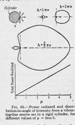
In this case the cylinder is the source, as it is in Werwolf's derivation. In my solution one would model a line of sources width b lying on a cylinder of radius a as a patch of sources that lies along phi = 0 and subtends an angle phi_0 about phi = 0 suck that b = sin( phi_0). This would then involve a Fourier series in phi and a sum of many modes m, but is certainly a reasonable thing to do.
This is actually done in Morse, Vibration and Sound, Sec. 26. The results are attached.
This is actually done in Morse, Vibration and Sound, Sec. 26. The results are attached.
Attachments
Last edited:
cylinder is the source
I always imagine an ideal cyclindrical source could be implemented (in the future) by moving a 4-dimensional cylinder in and out of the 3-D worl we live in (ignoring time). Or a point source as a 4-d sphere.
dave
gedlee ... thank you for your interest and contributions! So sorry you're not singing with Rush anymore (surely, i'm not the first ... )
Dr1v3n ... there are no stupid questions! Only stupid people (sorry couldn't resist ... certainly not you)
Thanks to everyone else as well but we must be careful ... although the geometry of an infinite line source certainly dictates a "cylindrical symmetry", this does NOT necessarily dictate or imply a "cylindrical wavefront" with 'ideal' characteristics (in time or frequency). For example, if the infinite line source excites with an ideal (time-domain) impulse, will we measure an impulse-like response (perhaps delayed and attenuated?) on an imaginary cylinder at some distance "r" from the line? OR, will there be some time-domain 'dispersion' of the impulse response ... while still obeying cylindrical symmetry? We'll soon see
(surely, i'm not the first ... )Dr1v3n ... there are no stupid questions! Only stupid people
(sorry couldn't resist ... certainly not you)Thanks to everyone else as well
but we must be careful ... although the geometry of an infinite line source certainly dictates a "cylindrical symmetry", this does NOT necessarily dictate or imply a "cylindrical wavefront" with 'ideal' characteristics (in time or frequency). For example, if the infinite line source excites with an ideal (time-domain) impulse, will we measure an impulse-like response (perhaps delayed and attenuated?) on an imaginary cylinder at some distance "r" from the line? OR, will there be some time-domain 'dispersion' of the impulse response ... while still obeying cylindrical symmetry? We'll soon see
Last edited:
POST #11
C. Infinite Line Source: frequency-domain pressure response (continued)
We've determined that our Infinite Line Source 'transfer function' is given by:
H(kr) = (-rho/4)*{Yo[kr] + j*Jo[kr]}
Bessel Functions ... don't offer much "insight" for the uninitiated
So let's look at the asymptotic behavior of our newly-derived 'transfer function', for small & large values of 'kr'
1. kr << 1
Jo[kr<<1] ~= 1
Yo[kr<<1] ~= (2/pi)*[ln[kr] - 0.1159315]
==>
H(kr<<1) ~= (rho/4)*{(2/pi)*[0.1159315 - ln[kr]] - j}
2. kr >> 1
Jo[kr>>1] ~= {SQRT[2/(pi*kr)]}*{cos[kr - (pi/4)]}
Yo[kr>>1] ~= {SQRT[2/(pi*kr)]}*{sin[kr - (pi/4)]}
==>
H(kr>>1) ~= (rho/4)*exp[-j*(pi/4)]*exp[-j*(kr)]*SQRT[2/(pi*kr)]
This last expression, the approximate/asymptotic behavior for large values of "kr", is VERY interesting we'll explore it in the next post
(yes i promise some charts/graphs of the frequency response are coming ...)
C. Infinite Line Source: frequency-domain pressure response (continued)
We've determined that our Infinite Line Source 'transfer function' is given by:
H(kr) = (-rho/4)*{Yo[kr] + j*Jo[kr]}
Bessel Functions ... don't offer much "insight" for the uninitiated
So let's look at the asymptotic behavior of our newly-derived 'transfer function', for small & large values of 'kr'
1. kr << 1
Jo[kr<<1] ~= 1
Yo[kr<<1] ~= (2/pi)*[ln[kr] - 0.1159315]
==>
H(kr<<1) ~= (rho/4)*{(2/pi)*[0.1159315 - ln[kr]] - j}
2. kr >> 1
Jo[kr>>1] ~= {SQRT[2/(pi*kr)]}*{cos[kr - (pi/4)]}
Yo[kr>>1] ~= {SQRT[2/(pi*kr)]}*{sin[kr - (pi/4)]}
==>
H(kr>>1) ~= (rho/4)*exp[-j*(pi/4)]*exp[-j*(kr)]*SQRT[2/(pi*kr)]
This last expression, the approximate/asymptotic behavior for large values of "kr", is VERY interesting
we'll explore it in the next post (yes i promise some charts/graphs of the frequency response are coming ...)
gedlee ... thank you for your interest and contributions! So sorry you're not singing with Rush anymore...
No ****. THE Geddy Lee.? Cheers!
POST #12
C. Infinite Line Source: frequency-domain pressure response (continued)
Before we explore our Infinite Line Source 'transfer function' for kr>>1 :
H(kr>>1) ~= (rho/4)*exp[-j*(pi/4)]*exp[-j*(kr)]*SQRT[2/(pi*kr)]
Let's examine this "kr" term in a little more detail ...
'k' is the so-called wavenumber, equal to w/c (where 'w' = radian frequency, and 'c' = speed of sound = 1100 ft/sec)
'r' is the distance from the Infinite Line Source to our measuring point
Therefore "kr" is really "distance divided by wavelength", and as such it's a unitless 'indicator' of how many wavelengths the measuring point is from the Infinite Line Source ... including a (favorable) '2pi' proportionality constant Here's some simple examples for kr=1 :
For a frequency of 100Hz (wavelength = 11 feet), kr=1 when r = 1.75 feet
For a frequency of 1kHz (wavelength = 1.1 feet), kr=1 when r = 0.175 feet
For a frequency of 10kHz (wavelength = 0.11 feet), kr=1 when r = 0.0175 feet
Note that larger values of "kr" will, of course, result for greater distances at any given frequency ... OR, for higher frequencies at any given distance For example, if we are measuring (or listening) at a distance of 8 feet from the Infinite Line Source, kr = 10 at a frequency of 219Hz ... and "kr" will be even larger at greater distances, or for higher frequencies.
So ... without providing a precise distinction (yet) between "near field" and "far field", we can expect that our approximate 'transfer function' for kr>>1 will be "reasonably useful" for a wide range of practical frequencies and distances (and, of course, we have the exact transfer function in our back pockets when kr>>1 doesn't apply)
Here's the approximate Infinite Line Source 'transfer function', for kr>>1, once again :
H(kr>>1) ~= (rho/4)*exp[-j*(pi/4)]*exp[-j*(kr)]*SQRT[2/(pi*kr)]
Let's look at these terms in detail :
rho/4 = proportionality constant. Let's just ignore it
exp[-j*(pi/4)] = constant phase shift (lag) of 45 degrees
exp[-j*(kr)] = linear phase shift, indicating the time-delay that corresponds to our measurement distance from the line
Comprehending ... and then quickly ignoring ... these terms, we are left with something i'll call the "normalized transfer function" for our Infinite Line Source (for large values of "kr") :
Hn(kr>>1) ~= SQRT[2/(pi*kr)]
The exploration of THIS simple expression is worthy of its very own post ... up next
C. Infinite Line Source: frequency-domain pressure response (continued)
Before we explore our Infinite Line Source 'transfer function' for kr>>1 :
H(kr>>1) ~= (rho/4)*exp[-j*(pi/4)]*exp[-j*(kr)]*SQRT[2/(pi*kr)]
Let's examine this "kr" term in a little more detail ...
'k' is the so-called wavenumber, equal to w/c (where 'w' = radian frequency, and 'c' = speed of sound = 1100 ft/sec)
'r' is the distance from the Infinite Line Source to our measuring point
Therefore "kr" is really "distance divided by wavelength", and as such it's a unitless 'indicator' of how many wavelengths the measuring point is from the Infinite Line Source ... including a (favorable) '2pi' proportionality constant
Here's some simple examples for kr=1 :For a frequency of 100Hz (wavelength = 11 feet), kr=1 when r = 1.75 feet
For a frequency of 1kHz (wavelength = 1.1 feet), kr=1 when r = 0.175 feet
For a frequency of 10kHz (wavelength = 0.11 feet), kr=1 when r = 0.0175 feet
Note that larger values of "kr" will, of course, result for greater distances at any given frequency ... OR, for higher frequencies at any given distance
For example, if we are measuring (or listening) at a distance of 8 feet from the Infinite Line Source, kr = 10 at a frequency of 219Hz ... and "kr" will be even larger at greater distances, or for higher frequencies.So ... without providing a precise distinction (yet) between "near field" and "far field", we can expect that our approximate 'transfer function' for kr>>1 will be "reasonably useful" for a wide range of practical frequencies and distances
(and, of course, we have the exact transfer function in our back pockets when kr>>1 doesn't apply)Here's the approximate Infinite Line Source 'transfer function', for kr>>1, once again :
H(kr>>1) ~= (rho/4)*exp[-j*(pi/4)]*exp[-j*(kr)]*SQRT[2/(pi*kr)]
Let's look at these terms in detail :
rho/4 = proportionality constant. Let's just ignore it
exp[-j*(pi/4)] = constant phase shift (lag) of 45 degrees
exp[-j*(kr)] = linear phase shift, indicating the time-delay that corresponds to our measurement distance from the line
Comprehending ... and then quickly ignoring ... these terms, we are left with something i'll call the "normalized transfer function" for our Infinite Line Source (for large values of "kr") :
Hn(kr>>1) ~= SQRT[2/(pi*kr)]
The exploration of THIS simple expression is worthy of its very own post ... up next
POST #13
C. Infinite Line Source: frequency-domain pressure response (continued)
Our 'normalized transfer function' for the Infinite Line Source (for kr>>1) is:
Hn(kr) ~= SQRT[2/(pi*kr)]
It's worth comparing this expression to a 'normalized transfer function' for the Point Source (developed around page 2, ignoring the time-delay and 'rho' scaling):
Hn(kr) = 1/(4pi*r)
Two interesting aspects of the 'transfer function' for the Point Source:
1. It's independent of frequency ... the frequency response magnitude, measured at any fixed point in space, is FLAT (no dependence on 'k' or 'w')
2. As we increase distance from the Point Source, the response falls off at 6dB for every doubling of distance
How does the Infinite Line Source compare (for kr>>1)? That "square root of 1/kr" relationship in the 'transfer function' tells us two things as well:
1. The frequency response magnitude measured at any fixed point in space is NOT flat ... in fact, it falls off at 3dB for every doubling of frequency
2. As we increase distance from the Infinite Line Source, the response falls off at only 3dB for every doubling of distance
While the first point is rather unfortunate, and would ultimately call for some sophisticated equalization (FIR much preferred, since 3dB/octave is challenging with IIR) and healthy dynamic range in the driving electronics (assuming we can actually build something like an "infinite" line source turns out, we can! ) ... that second point is a HUGE plus (in my humble opinion). For example, a response that drops off at only 3dB per doubling-distance has wonderful implications for a wider sweet spot when a pair of line sources are employed for stereo listening
It's worth noting that ALL of this has been done, well before me. If i can claim anything at all innovative, so far, it may only be my 'transfer function' view of this domain of acoustics. Also, i certainly expect more pros & cons to be debated as the thread develops but next i must do my best to present a frequency response chart of the 'transfer function' for the Infinite Line Source ...
C. Infinite Line Source: frequency-domain pressure response (continued)
Our 'normalized transfer function' for the Infinite Line Source (for kr>>1) is:
Hn(kr) ~= SQRT[2/(pi*kr)]
It's worth comparing this expression to a 'normalized transfer function' for the Point Source (developed around page 2, ignoring the time-delay and 'rho' scaling):
Hn(kr) = 1/(4pi*r)
Two interesting aspects of the 'transfer function' for the Point Source:
1. It's independent of frequency ... the frequency response magnitude, measured at any fixed point in space, is FLAT (no dependence on 'k' or 'w')
2. As we increase distance from the Point Source, the response falls off at 6dB for every doubling of distance
How does the Infinite Line Source compare (for kr>>1)? That "square root of 1/kr" relationship in the 'transfer function' tells us two things as well:
1. The frequency response magnitude measured at any fixed point in space is NOT flat ... in fact, it falls off at 3dB for every doubling of frequency
2. As we increase distance from the Infinite Line Source, the response falls off at only 3dB for every doubling of distance
While the first point is rather unfortunate, and would ultimately call for some sophisticated equalization (FIR much preferred, since 3dB/octave is challenging with IIR) and healthy dynamic range in the driving electronics (assuming we can actually build something like an "infinite" line source
turns out, we can! ) ... that second point is a HUGE plus (in my humble opinion). For example, a response that drops off at only 3dB per doubling-distance has wonderful implications for a wider sweet spot when a pair of line sources are employed for stereo listening It's worth noting that ALL of this has been done, well before me. If i can claim anything at all innovative, so far, it may only be my 'transfer function' view of this domain of acoustics. Also, i certainly expect more pros & cons to be debated as the thread develops
but next i must do my best to present a frequency response chart of the 'transfer function' for the Infinite Line Source ...
Last edited:
POST #14
C. Infinite Line Source: frequency-domain pressure response (continued)
The exact transfer function for the Infinite Line Source, for any value of "kr", is :
H(kr) = (-rho/4)*{Yo[kr] + j*Jo[kr]}
where :
Jo[x] is the zero-order Bessel Function of the 1st kind
Yo[x] is the zero-order Bessel Function of the 2nd kind
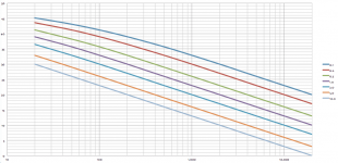
Let's chart the magnitude response, as a function of both distance and frequency (normalized so that the farthest distance and highest frequency is 0dB), described by this frequency-domain 'transfer function' :
-------20Hz---50Hz---100Hz--200Hz-500Hz--1kHz---2kHz---5kHz---10kHz--20kHz
0.1M 45.2dB 43.1dB 41.2dB 39.0dB 35.7dB 32.9dB 30.0dB 26.0dB 23.0dB 20.0dB
0.2M 43.6dB 41.2dB 39.0dB 36.5dB 32.9dB 30.0dB 27.0dB 23.0dB 20.0dB 17.0dB
0.5M 41.2dB 38.2dB 35.7dB 32.9dB 29.0dB 26.0dB 23.0dB 19.0dB 16.0dB 13.0dB
1.0M 39.0dB 35.7dB 32.9dB 30.0dB 26.0dB 23.0dB 20.0dB 16.0dB 13.0dB 10.0dB
2.0M 36.5dB 32.9dB 30.0dB 27.0dB 23.0dB 20.0dB 17.0dB 13.0dB 10.0dB 07.0dB
5.0M 32.9dB 29.0dB 26.0dB 23.0dB 19.0dB 16.0dB 13.0dB 09.0dB 06.0dB 03.0dB
10.M 30.0dB 26.0dB 23.0dB 20.0dB 16.0dB 13.0dB 10.0dB 06.0dB 03.0dB 00.0dB
Notes :
- The left-most column is distance, in meters (M), from the line source.
- The value of "kr" for each data point can be found by multiplying the distance (in meters) by the frequency (in Hz), and scaling by 2pi/c = 0.0184 seconds/meter.
- The "3dB per octave", and "3dB per doubling-distance", rules become quickly apparent as "kr" exceeds unity.
And so ends our frequency-domain pressure response discussion, for the Infinite Line Source up next, the derivation of the time-domain impulse response for the Infinite Line Source ...
C. Infinite Line Source: frequency-domain pressure response (continued)
The exact transfer function for the Infinite Line Source, for any value of "kr", is :
H(kr) = (-rho/4)*{Yo[kr] + j*Jo[kr]}
where :
Jo[x] is the zero-order Bessel Function of the 1st kind
Yo[x] is the zero-order Bessel Function of the 2nd kind
Let's chart the magnitude response, as a function of both distance and frequency (normalized so that the farthest distance and highest frequency is 0dB), described by this frequency-domain 'transfer function' :
-------20Hz---50Hz---100Hz--200Hz-500Hz--1kHz---2kHz---5kHz---10kHz--20kHz
0.1M 45.2dB 43.1dB 41.2dB 39.0dB 35.7dB 32.9dB 30.0dB 26.0dB 23.0dB 20.0dB
0.2M 43.6dB 41.2dB 39.0dB 36.5dB 32.9dB 30.0dB 27.0dB 23.0dB 20.0dB 17.0dB
0.5M 41.2dB 38.2dB 35.7dB 32.9dB 29.0dB 26.0dB 23.0dB 19.0dB 16.0dB 13.0dB
1.0M 39.0dB 35.7dB 32.9dB 30.0dB 26.0dB 23.0dB 20.0dB 16.0dB 13.0dB 10.0dB
2.0M 36.5dB 32.9dB 30.0dB 27.0dB 23.0dB 20.0dB 17.0dB 13.0dB 10.0dB 07.0dB
5.0M 32.9dB 29.0dB 26.0dB 23.0dB 19.0dB 16.0dB 13.0dB 09.0dB 06.0dB 03.0dB
10.M 30.0dB 26.0dB 23.0dB 20.0dB 16.0dB 13.0dB 10.0dB 06.0dB 03.0dB 00.0dB
Notes :
- The left-most column is distance, in meters (M), from the line source.
- The value of "kr" for each data point can be found by multiplying the distance (in meters) by the frequency (in Hz), and scaling by 2pi/c = 0.0184 seconds/meter.
- The "3dB per octave", and "3dB per doubling-distance", rules become quickly apparent as "kr" exceeds unity.
And so ends our frequency-domain pressure response discussion, for the Infinite Line Source
up next, the derivation of the time-domain impulse response for the Infinite Line Source ...Let's chart the magnitude response, as a function of both distance and frequency
dave
Attachments
- Status
- This old topic is closed. If you want to reopen this topic, contact a moderator using the "Report Post" button.
- Home
- Loudspeakers
- Multi-Way
- Infinite Line Source: analysis