Hornresp Update 5000-190505
Hi Everyone,
BUG FIX 1
The stubbed horn acoustical impedance chart was not being displayed. This has now been fixed.
BUG FIX 2
Stubbed horn system volumes were not correct. This has now been fixed.
BUG FIX 3
The inconsistency in results detailed in Post #9490 has now been resolved. My thanks to Damien for identifying the issue.
BUG FIX 4
Problems using the Driver Arrangement tool, resulting from the addition of the stubbed horn SH1, SH2, SH3 and SH4 options, and reported by a user via email, have now been fixed.
CHANGE 1
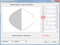
The flare of a throat adaptor in a stubbed horn design can now be changed in the Loudspeaker Wizard. My thanks to Damien for his Post #9508 identifying this oversight.
CHANGE 2
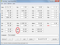
The flare of an absorber chamber port can now be changed on the Input Parameters window and in the Loudspeaker Wizard (specify Lp or Cyl if a standard cylindrical port is required). The two attachments refer.
Kind regards,
David
Hi Everyone,
BUG FIX 1
The stubbed horn acoustical impedance chart was not being displayed. This has now been fixed.
BUG FIX 2
Stubbed horn system volumes were not correct. This has now been fixed.
BUG FIX 3
The inconsistency in results detailed in Post #9490 has now been resolved. My thanks to Damien for identifying the issue.
BUG FIX 4
Problems using the Driver Arrangement tool, resulting from the addition of the stubbed horn SH1, SH2, SH3 and SH4 options, and reported by a user via email, have now been fixed.
CHANGE 1
The flare of a throat adaptor in a stubbed horn design can now be changed in the Loudspeaker Wizard. My thanks to Damien for his Post #9508 identifying this oversight.
CHANGE 2
The flare of an absorber chamber port can now be changed on the Input Parameters window and in the Loudspeaker Wizard (specify Lp or Cyl if a standard cylindrical port is required). The two attachments refer.
Kind regards,
David
Attachments
We'll revive it
That's the spirit!
hi David - in the sim of a 12" diameter flat baffle (maybe that's not correct ?) vs 12" diameter oblate spheroid, spl is always lile 12dB greater for the waveguide up to 20KHz and 30 off axis. Am I missing something in thinking they should be more alike up high in frequency and off axis ? (sorry for the stupid question)
https://i.imgur.com/evKnih9.png
https://i.imgur.com/evKnih9.png
in the sim of a 12" diameter flat baffle vs 12" diameter oblate spheroid
Hi Fred,
As far as Hornresp is concerned, you are comparing a conical horn of axial length 0.1 cm to an oblate spheroidal waveguide of axial length 10.16 cm. The theoretical power and pressure responses of the two systems will be quite different.
Using a very short horn to approximate a direct radiator in an open baffle will not give particularly satisfactory results. There are limits on how far you can "push the envelope" with the Hornresp models
") .
.Kind regards,
David
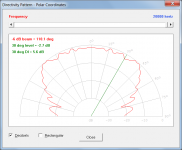
David - when comparing a 3 inch fullrange on two "similar size" horns, the oblate-spheroid horn shows similar power to the equivalent size exponential horn yet the oblate spheroid is showing 100 degrees beamwidth all the way to 20KHz while the exponential horn has narrowed to `42 degrees by 10KHz and 30 degrees beamwidth by 20KHZ. Why would they be so different? When examining such a horn/driver case with hornresp, should one perhaps limit how high to examine for realistic result?
the 100 degrees indicates constant directivity characteristics (?) while the exponential is progressively beaming.
I'm apparently misunderstanding a fair amount ;^(


the 100 degrees indicates constant directivity characteristics (?) while the exponential is progressively beaming.
I'm apparently misunderstanding a fair amount ;^(
Last edited:
Why would they be so different?
Hi Fred,
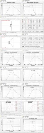
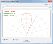
As advised on previous occasions, the Hornresp directivity models are relatively simple, and the results should be considered as indicative only. An exponential horn will "beam" at higher frequencies whereas an OSW acts more like a conical horn in that it will exhibit constant directivity characteristics. This is what Hornresp attempts to show - see the attached comparison using your two test example horns.
In reality the 3" driver diaphragm will not act as rigid piston up to 20KHz anyway, so the actual pressure response will be somewhat different, regardless of what any predictions may suggest.
You would really need to use full-blown finite element analysis techniques to accurately predict the pressure response. Calculations would take several hours to complete if you wanted to fully analyse up to 20Khz. I don't have the patience for that - I have the attention span of a mosquito
.Kind regards,
David
Attachments
As David explained, the Hornresp directivity models are quite simple. To properly calculate the directivity of a horn, you need to know the distribution of particle velocity at the mouth (iow, the shape of the wave front), and for that you also need a more complex model of the horn itself. So Hornresp isn't really suited to tweaking the horn shape for high frequency directivity optimisation.
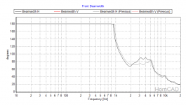
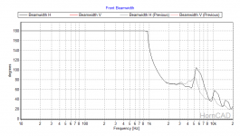
I simulated the directivity of your two horns using the Mode Matching Method, assuming the horn is mounted in an infinite baffle (no, or finite, baffle would require diffraction modelling, which I haven't fully implemented yet). They are not very different. Which isn't that surprising when you compare the profiles.
Below about 1.5kHz, neither horn can control directivity, and they behave the same. Above 5kHz, the large throat takes over control, and they behave the same. You have a small range where they are different. See Attachment 1.
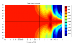
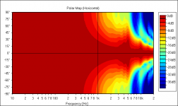
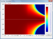
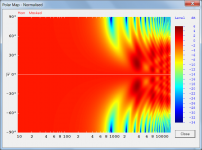
The normalized polar maps also show that the OS has more of an on-axis dip. See Attachments 2 and 3 (Exp and OS)
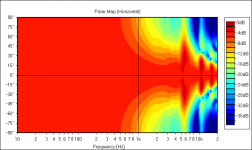
Since the driver is smaller than the horn throat, it will excite modes here, which will mess up directivity some more. See Attachments 4 and 5, these are for the exponential horn with a 32cm2 piston source driving the 45cm2 throat.
Also you have the complication of the shape of the cone and the breakup modes of the diaphragm. Now we are getting into the domain of fully coupled FEA...
I simulated the directivity of your two horns using the Mode Matching Method, assuming the horn is mounted in an infinite baffle (no, or finite, baffle would require diffraction modelling, which I haven't fully implemented yet). They are not very different. Which isn't that surprising when you compare the profiles.
Below about 1.5kHz, neither horn can control directivity, and they behave the same. Above 5kHz, the large throat takes over control, and they behave the same. You have a small range where they are different. See Attachment 1.
The normalized polar maps also show that the OS has more of an on-axis dip. See Attachments 2 and 3 (Exp and OS)
Since the driver is smaller than the horn throat, it will excite modes here, which will mess up directivity some more. See Attachments 4 and 5, these are for the exponential horn with a 32cm2 piston source driving the 45cm2 throat.
Also you have the complication of the shape of the cone and the breakup modes of the diaphragm. Now we are getting into the domain of fully coupled FEA...
Attachments
I simulated the directivity of your two horns using the Mode Matching Method, assuming the horn is mounted in an infinite baffle
Thanks Bjørn.
Your implemention of the Mode Matching Method obviously doesn't require several hours to produce a meaningful result
.Kind regards,
David
Thanks David and Kolbrek for the discussion. I probably should have not brought up the subject but curious of what can and can't be discerned with the upper reaches of hornresp.
I would like to see analysis of a certain enclosure but know its considered nonsensical
https://i.imgur.com/2XyfW19.png
I would like to see analysis of a certain enclosure but know its considered nonsensical
https://i.imgur.com/2XyfW19.png
The normalized polar maps also show that the OS has more of an on-axis dip. See Attachments 2 and 3 (Exp and OS)
Just to compare, the Hornresp-generated equivalents are attached - clearly quite different
.Attachments
Hi Fred,
It's no secret that Hornresp is definitely more comfortable when calculating the power responses of bass horn systems, rather than attempting to predict high-frequency off-axis pressure responses of mid-range and high-frequency horns.
You are not going to see it analysed in Hornresp, that's for sure....
Kind regards,
David
curious of what can and can't be discerned with the upper reaches of hornresp.
It's no secret that Hornresp is definitely more comfortable when calculating the power responses of bass horn systems, rather than attempting to predict high-frequency off-axis pressure responses of mid-range and high-frequency horns
.I would like to see analysis of a certain enclosure but know its considered nonsensical
You are not going to see it analysed in Hornresp, that's for sure...
.Kind regards,
David
Hi Fred,
As advised on previous occasions, the Hornresp directivity models are relatively simple, and the results should be considered as indicative only.
Perhaps if there was some way to indicate on the Hornresp-produced charts at what point the accuracy of the simplified sim should be questioned.
With line graphs, this could be done by replacing the solid line with a dotted line above the frequency at which the deviation may be significant. I'm not sure what could be done in the polar maps though - maybe a dotted vertical line at the frequency where the deviation may be significant..?
It's no secret that Hornresp is definitely more comfortable when calculating the power responses of bass horn systems, rather than attempting to predict high-frequency off-axis pressure responses of mid-range and high-frequency horns
Kind regards,
David
Hence, we are in the Subwoofer forum of diyaudio!
Perhaps if there was some way to indicate on the Hornresp-produced charts at what point the accuracy of the simplified sim should be questioned.
Hi Brian,
The accuracy of the Hornresp pressure response predictions is influenced by the size of the horn. In most cases, the results for relatively long horns with relatively small throats seem to be better than those for relatively short horns with relatively large throats, such as those used in Fred's test examples. It is not possible to set hard and fast rules because the particular flare profile used is also a factor. The directivity tools were included in Hornresp primarily as an educational aid to enable users to see how directivity characteristics affect the response in general. As Bjørn mentioned, the Hornresp models do not know the particle velocity distribution at the horn mouth, so it is prudent not to expect too much from them
.Kind regards,
David
Your implemention of the Mode Matching Method obviously doesn't require several hours to produce a meaningful result
No, these results took only about 4 seconds to compute (500 frequencies, 32 modes). But I'm cheating a little, as I use (6 thread) parallel computing
No, these results took only about 4 seconds to compute (500 frequencies, 32 modes). But I'm cheating a little, as I use (6 thread) parallel computing
I suspect that it would not even be possible to run a MMM simulation of 500 frequencies and 32 modes on my computer, let alone worrying about the time that it might take
.(My PC has an AMD E-450 processor and 2 GB RAM, of which only 1.6 GB is usable).
I can see now that what I really need is a quantum computer, or a Cray supercomputer at the very least! The Cray pictured in the attachment below would probably cope okay - it has the following specification:
Manufacturer: Cray Inc. (USA)
Model: XC40 Series Supercomputer
Compute Processors: Intel Xeon E5-2690V3 “Haswell” processors (12-core, 2.6 GHz)
Computing Power: 1,097 TeraFLOPS (1 PetaFLOP+).
Memory: 93 Terabytes (64 GB of DDR4-2133 per compute node).
Interconnect: Cray Aries interconnect, at 72 gigabits/sec per node
Network Topology: Cray Dragonfly – 56% populated
Nodes: 1488 (35,712 processor cores, two compute processors per node)
Weight: 1.7 tonnes/cabinet
Power consumption: circa. 50 kWatts/cabinet
Local storage: Sonexion 1600 Data Storage System, 3 Petabytes, w/ 70 GB/sec sustained r/w performance
Attachments

- Home
- Loudspeakers
- Subwoofers
- Hornresp