Kindhornman, I don't think or believe the dip at ~70 Hz is an error from REW. You've got to remember DRC is a correction suite, not a measurement suite. It has dip limiting, also ignoring non minimum phase behaviour for this window etc. It's parameter driven to make certain judgement calls.
The smoothing from DRC will be about 1/3 octave on the frequency dependant window. That's a completely different picture from smoothing a 500 ms window with 1/3 octave.
Nor will it be the same as a REW FDW window with more cycles, it will only look more similar.
Why do I say 1/3 octave? Because DRC covers exactly 30 steps from 20 Hz to 20 KHz, all on 1/3 octave key points. But you've got to keep in mind that there's more going on in DRC to make that "slice" of the impulse. It's task is not to show a measurement in any kind of precision. It's meant to correct the frequency response but ignore certain things like huge dips, non minimum phase behaviour etc.
REW's frequency dependant window probably is more coarse than that 1/3 octave smoothing. So it will be more limited in use to make judgement calls. If we look at the second plot it seems DRC and REW aren't too far off. Except the dips shown in REW are a lot deeper in DRC's plot. Which probably means the big dip that REW shows in my first plot is exceeding certain parameters in DRC. You don't want to boost a null.
Minimum phase section in the DRC-FIR documentation:
No dip filtering yet, but a lot of variables to determine it's behaviour. It's up to the user to make the choices. Or leave it at default values...
I've only played with some of them to make a better match between what I hear and how it's corrected. Very different from wanting to "see" the curve.
The only point in all this, for me is to be aware of the differences. They are larger than I expected them to be. That is valid information and use it any way you like. The plots above were made with a 5-cycle template provided by gmad in the convolution thread. I did not change any values prior to making the plots.
DRC-FIR documentation said:6.4 MP - Minimum phase Prefiltering
6.4.1 MPPrefilterType
This parameter can be either B for the usual band windowing prefiltering stage or S for the sliding lowpass method. The first method splits the input response into log spaced bands and window them depending on some parameters but basically with a window length which decrease exponentially with the center frequency of the band. The sliding lowpass method instead filters the impulse response with a time varying lowpass filter with a cutoff frequency which decreases exponentially with the sample position with respect to the time axis zero. This last one is a stepless procedure.
Using either a lowercase b or s for the MPPrefilterType parameters enable the single side version of the prefiltering procedures. The procedure is applied starting from the impulse center, leaving the first half of the impulse response unchanged. This gives less pre-echo artifacts, and should be used when the pre-echo truncation inversion procedure is used. Please remember to set the prefiltering parameters to values which are adequate for the procedure used.
6.4.2 MPPrefilterFctn
This parameter sets the type of prefiltering function used, i.e. P for the usual inverse proportional function, or B for the bilinear transform based prefiltering function. For a comparison between the two functions see figure 6. The default is B.
6.4.3 MPWindowGap
This parameter changes a little the window function (Blackman) used for the band windowing prefiltering stage. It sets a small flat unitary gap, whose length is expressed in samples, at the center of the window function, so that even if the impulse center is slightly misaligned with respect to the time axis zero there is no high frequency overcorrection. For band windowing prefiltering procedure usually this overcorrection is in the order of 0.1 − 0.2 dB at 20 kHz for errors of 2 to 3 samples, so it is not important at all in real world situations, but if you want to fix even this small problem this parameter lets you do it.
MPWindowGap should never be more than 2 sample less than MPUpperWindow and it is usually no more than few samples (5 to 10). If in any situation it is bigger than the calculated window DRC automatically reduces the gap to 2 less than the applied window. When MPWindowGap is 0 DRC behaves exactly as in the older versions. For the sliding lowpass procedure this sets just the window gap used for the initial windowing before the procedure starts.
6.4.4 MPLowerWindow (*)
Length of the window for the minimum phase component prefiltering at the bottom end of the frequency range. Longer windows cause DRC to try to correct a longer part of the impulse response but cause greater sensibility to the listening position. Typical values are between 16384 and 65536. MPLowerWindow must not be greater than BCInitWindow.
6.4.5 MPUpperWindow (*)
Length of the window for the minimum phase component prefiltering at the upper end of the frequency range. Longer windows cause DRC to try to correct a longer part of the impulse response but cause greater sensibility on the listening position. Typical values are between 22 and 128. MPUpperWindow must be not greater than MPLowerWindow, and usually is much shorter than that.
6.4.6 MPStartFreq
Start frequency for the prefiltering stage. Usually 20 Hz or just something less.
6.4.7 MPEndFreq
End frequency for the prefiltering stage. Usually set at 20 kHz, i.e. 20000. Of course you must be using a sample rate which is greater than 40 kHz to set this above 20 kHz.
6.4.8 MPWindowExponent (*)
This is the exponent used in the frequency dependent window length computation for the band windowing procedure, or in the computation of the time dependent cutoff frequency for the sliding lowpass procedure.
The window length for band windowing is computed with the following expression:
W =
1
____________
A * (F + Q) WE
Where W is the window length, F is the normalized frequency, WE is the window exponent, A and Q are computed so that W is equal to MPLowerWindow at MPStartFreq and is equal to MPUpperWindow at MPEndFreq. If you set MPLowerWindow equal to the value used for MPInitWindow in DRC 1.2, set MPWindowExponent to the same value of version 1.2 and set MPUpperWindow to the value you got at the upper limit of the frequency range in version 1.2 you should get results much similar to the 1.2 DRC release.
In a similar way the cutoff frequency for the sliding lowpass prefiltering stage is computed with:
F =
1
_____________
A * (W + Q) WE
with identical parameters but reversed perspective, i.e. the cutoff frequency is computed from the window length and not the other way around. In both cases W and F are considered normalized between 0 and 1.
These parametric functions are used when the proportional function is selected using the MPPrefilterFctn (see section 6.4.2) parameter. The parametric functions derived from the bilinear transformation are quite different and more complicated, so they aren’t explained here.
Changing the window exponent provides different prefiltering curves, see section 4.2 for a deeper explanation. Increasing the window exponent gives higher correction in the midrange. Typical values are between 0.7 and 1.2.
6.4.9 MPFilterLen
Filter length, in taps, used to perform band splitting or sliding lowpass prefiltering of the input signal. Higher values give better filter resolution but require a longer computation. Typical values for band windowing are between 4096 and 65536. Sometimes may be useful to use short filters (64 - 512 taps) to get a more “fuzzy” correction at lower frequencies.
With the sliding lowpass procedure similar filters should be used. Usually the filter length is in the 512 - 65536 range. Short filters (16 - 64 taps) gives a similar fuzzy correction at the bottom end, but with a different behaviour than band windowing.
6.4.10 MPFSharpness (*)
This parameter applies only to the sliding lowpass prefiltering procedure and control the sharpness of the filtering performed in the filtered region of the time-frequency plane. A value of 1.0 provides the same behaviour of version 2.3.1 of DRC and provides the maximum allowable filtering sharpness without affecting the direct sound, but also creates a substantial amount of spectral spreading in the filter transition region of the time-frequency plane. Values above 1.0 increase the spectral spreading up to a point where it starts affecting also the direct sound, with the introduction of some ripple in the direct sound itself. Values below 1.0 reduce the spectral spreading in the filtered region at the expense of a little reduction in the filter sharpness. Typical values for this parameter are between 0.1 and 0.75, with a default value of 0.25.
6.4.11 MPBandSplit
Fractional octave splitting of band windowing. Band windowing is performed in 1 / MPBandSplit of octave bands. Usual values are between 2 and 6. The higher this value the higher should be MPFilterLen. Values greater than 6 usually give no improvements.
For the sliding lowpass prefiltering this just gives the rate at which log messages are reported during the prefiltering procedure and has no effect on the prefiltering procedure itself, which is always stepless.
6.4.12 MPHDRecover
After prefiltering the minimum phase component may be no longer minimum phase, with a bit of excess phase component added. Setting this parameter to Y enable a second homomorphic deconvolution on the prefiltered minimum phase component to make it minimum phase again. This is important especially if the pre-echo truncation inversion procedure is used. This procedure assumes that the minimum phase part really is minimum phase, so skipping this step may cause it to fail in avoiding pre-echo artifacts.
6.4.13 MPEPPreserve
Setting this to Y causes the excess phase part of the filtered impulse response to be preserved after the MPHDRecover step. This excess phase part is then convolved with the excess phase part of the filtered impulse response to preserve it and invert it. This provides a slight improvement in the direct sound phase response. The default value is Y.
6.4.14 MPHDMultExponent
Exponent of the multiplier of the FFT size used to perform the homomorphic deconvolution described above. The FFT size used is equal to the first power of two greater than or equal to MPPFFinalWindow * (2 MPHDMultExponent). Higher exponents give more accurate results, but require a longer computation. Usually a value of 2 or 3 is used. If this parameter is less than 0 no multiplier will be used. Be careful because if the FFT size isn’t a power of two the procedure can take a long time to complete.
6.4.15 MPPFFinalWindow
Final window of the prefiltering stage. Usually the same as MPLowerWindow or just something more. If set to 0 no windowing is applied.
6.4.16 MPPFNormFactor
Normalization factor for the minimum phase component after prefiltering. Usually 0.
6.4.17 MPPFNormType
Normalization type for the minimum phase component after windowing. Usually E.
6.4.18 MPPFOutFile
Output file for the minimum phase component after band windowing. Usually not used (commented out).
6.4.19 MPPFOutFileType
Output file type for the minimum phase component after windowing. D = Double, F = Float, I = Integer.
No dip filtering yet, but a lot of variables to determine it's behaviour. It's up to the user to make the choices. Or leave it at default values...
I've only played with some of them to make a better match between what I hear and how it's corrected. Very different from wanting to "see" the curve.
The only point in all this, for me is to be aware of the differences. They are larger than I expected them to be. That is valid information and use it any way you like. The plots above were made with a 5-cycle template provided by gmad in the convolution thread. I did not change any values prior to making the plots.
Last edited:
The smoothing from DRC will be about 1/3 octave on the frequency dependant window. That's a completely different picture from smoothing a 500 ms window with 1/3 octave.
Nor will it be the same as a REW FDW window with more cycles, it will only look more similar.
Why do I say 1/3 octave? Because DRC covers exactly 30 steps from 20 Hz to 20 KHz, all on 1/3 octave key points. But you've got to keep in mind that there's more going on in DRC to make that "slice" of the impulse. It's task is not to show a measurement in any kind of precision. It's meant to correct the frequency response but ignore certain things like huge dips, non minimum phase behaviour etc.
REW's frequency dependant window probably is more coarse than that 1/3 octave smoothing. So it will be more limited in use to make judgement calls. If we look at the second plot it seems DRC and REW aren't too far off. Except the dips shown in REW are a lot deeper in DRC's plot. Which probably means the big dip that REW shows in my first plot is exceeding certain parameters in DRC. You don't want to boost a null.
Scrap this comment... as the windowing I used is based on the sliding window (MPPrefilterType=s) it only reports the steps given in the value MPBandSplit. As that value has been set to 3 it will only report 1/3 octave numbers in the log file, while the actual sliding window is without such steps. (should have remembered that! Even if it was a while ago that I looked into it) I could set it to "b" and 1/3 to see if that resembles what REW is getting.
To touch on the differences as seen between REW and DRC again: I've said on this thread that I looked for parameters that gave me a correction where I wanted it, and leave certain things untouched. That's exactly what you see DRC do here. That does not mean there is no dip at 70 Hz. It only means DRC is doing what it is told to do.
After all, it is part of a correction procedure and not a measuring suite.
My only surprise was the difference between the implementation in REW compared to DRC. Greg has said to find the same results and may even have posted about it on the convolution thread?
In DRC you can actually choose the variables that determine the behaviour. In other words choose what you allow to be corrected. REW only shows the result and I would have liked to have more resolution. I could ask for that, but where does it end? One user might want the resolution we have already while another might want much more course data. I can live with the current situation as I was used to doing things a bit different already. It gives me plenty of solid ground to determine my desired outcome. Just as long as you do not use DRC as a measurement suite
") .
.I have noticed it too. You basically have to double the freq dependent window length with REW relative to DRC to get similar looking results...
While that will make it look similar, you would be looking at another "point in time" on the graph. My guess is REW is using 1/x octave smoothing with the "x" depending on the length of the frequency dependant window. DRC is using a step less sliding window in my presented graphs.
Last edited:
I could set it to "b" and 1/3 to see if that resembles what REW is getting.
Quoting myself again... hmmm
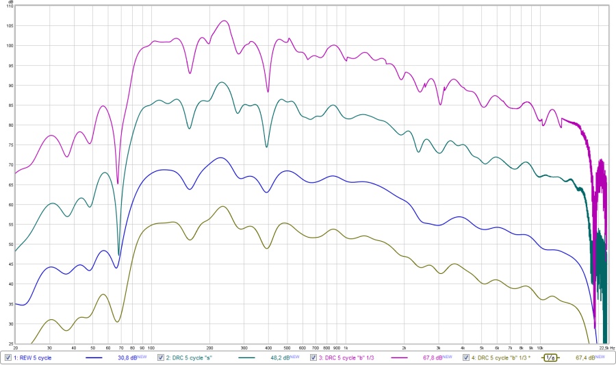
The top graph is DRC doing a 1/3 octave 5 cycle window. (MPPrefilterType = b and MPBandSplit = 3)
Second one is DRC's sliding window (my favourite)
Third graph is REW's 5 cycle window
Fourth graph is DRC's 1/3 octave 5 cycle window we saw, but smoothed 1/6 octave.
In hindsight I see why, knowing the result of the first type of a frequency dependant window that was introduced in REW. Well, this satisfies all of my curiosity.
case closed?
You might want to ask John Mulcahy (REW author) for help. He might be able to clear it up or maybe even get the correct functionality in REW so we don't need to learn another program.
The trouble is, what is the correct procedure? The first implementation in REW was a psychoacoustic window, based on a fixed mix of values in number of cycles used and had a ~ 1/12 octave smoothing look. I still have that REW version saved on my HD as that window disappeared later on.
Last edited:

REW does allow smoothing on top of FDW, IIRC by default it adds 1/48 smoothing as soon as you activate FDW. FDW in REW is also v sensitive to the position of the window ref time. Have you checked that?Well REW does not offer anything else at this time, no smoothing parameters. Just a setting in the IR box. I caught this today while looking at measurements from someone else. I haven't used it in my project as it wasn't available yet. That deviation at ~70 Hz is strange. For now I'll put my trust in DRC-FIR. Don't make too much of this example, it's only meant as an example. Just know the results from REW are smoothed when using frequency dependant windows. They sure looked that way, but I noticed some bigger deviations or detail changes that made me look and post about it.
My nickname could almost be Mr. FDW thus I wanted to tell you guys as soon as I found out.
P.S. Even the DRC window will be smoothed, the question would be: how much...
Last edit today: one big difference would be: the DRC result is a minimum phase generated view. So to see how it would look in REW, You'd need to export the impulse with "Export Min Phase version of IR" selected, re-import and compare using the FDW. That won't make it more detailed though. Just be warned I guess...
There are certainly differences between the different implementations anyway, acourate FDW looks different to REW which looks slightly different to Holm (and which seems to be different to that used by DRC as well). Nice to have options
More smoothing would move us further in the wrong direction as you are probably aware of. Yes I did notice the position of the windows ref time being of influence, as it should be.REW does allow smoothing on top of FDW, IIRC by default it adds 1/48 smoothing as soon as you activate FDW. FDW in REW is also v sensitive to the position of the window ref time. Have you checked that?
There are certainly differences between the different implementations anyway, acourate FDW looks different to REW which looks slightly different to Holm (and which seems to be different to that used by DRC as well). Nice to have options
True, I have not tried all of them but as long as I can find my way around the ones I use I'm not worried. Just use more than one solution to verify what it is you're doing. Easier said than done though. I briefly played with Audiolense as a measurement suite. Even more will be available of coarse.
I still prefer FDW to a fixed value gate. Just not this particular implementation.
I was just about to jump on the TC9 sale and on the arrays bandwagon!
I figured that I was going to save almost the price of shipping to here...
But...
The same day, we found and bought a VW van! I'll be turning it into a surfing-camper, so funds that were supposed to go to the new arrays will probably be diverted to setting up the van!
Sorry guys, my arrays will have to wait... again!
Back to regular posting about tweaks and stuff now...
Attachments

Wesayso,
Thanks for your in-depth explanation of the differences between the two original graphs. I guess the bottom line really was that we were looking at two different things. One just a measurement and the other a correction for the room. Apples and oranges really. If we were looking for a simple room measurement without correction from any two measurement systems I would want to see a lot better correlation with similar smoothing.
Thanks for your in-depth explanation of the differences between the two original graphs. I guess the bottom line really was that we were looking at two different things. One just a measurement and the other a correction for the room. Apples and oranges really. If we were looking for a simple room measurement without correction from any two measurement systems I would want to see a lot better correlation with similar smoothing.
It would take a lot less TC9's to make floor to ceiling arrays in the van!
Indeed! Very true!
That's one way of looking at it!
Wesayso,
Thanks for your in-depth explanation of the differences between the two original graphs. I guess the bottom line really was that we were looking at two different things. One just a measurement and the other a correction for the room. Apples and oranges really. If we were looking for a simple room measurement without correction from any two measurement systems I would want to see a lot better correlation with similar smoothing.
Close, but not quite. The graph (that's not shown in regular use) from DRC is the foundation upon which DRC is going to base it's correction. It is achieved by extracting the minimum phase version with a length(*) set by user for the frequency dependant window which extracts this info out of a regular impulse. Just one short stop in DRC. There are others that make up the whole correction procedure. Another separate frequency dependant window (with it's own settings) is performing a similar action to determine the excess phase. Many more steps involved. But the one I showed is already a "set view". Meaning the one that sets al parameters is responsible for the outcome of that view.
(*) this length is completely variable. The one used here is 5 cycles over the entire frequency spectrum of 20 Hz to 20 KHz.
The sliding window seems to have a clear advantage in resolution. It will still average to a certain degree compared to a 500 ms unsmoothed plot. REW's implementation is still developing (I hope). It was a request by Bob Katz that set it's development in motion (probably more requests have been filed previously): Feature Request: Frequency Dependent Windowing - Home Theater Forum and Systems - HomeTheaterShack.com
Wow, that was fast...
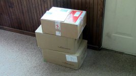
Had quite the deliveries today
Actually, I was surprised all 64 of them TC9s fit in those two boxes (one was only half full).
The box on top are the two SMPS I ordered from Hypex for my First One build.
Efficient packaging of the TC9s...
Had quite the deliveries today
Actually, I was surprised all 64 of them TC9s fit in those two boxes (one was only half full).
The box on top are the two SMPS I ordered from Hypex for my First One build.
Efficient packaging of the TC9s...
Attachments

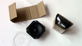
TC9 compared to the 10F
Most of You have seen the TC9
But for laughs and giggles, lets look at it side by side, to the ScanSpeak 10F:
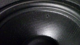
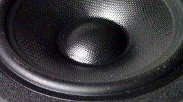
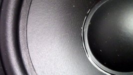
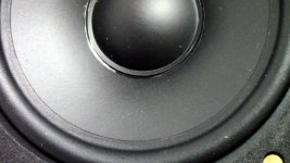
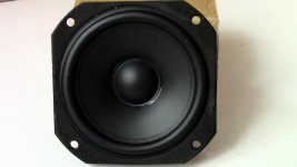
Here are the cones: First three photos are the TC9, last two are the 10F
Both are finished quite well. The TC9 almost looks like a poly cone, I have never seen a paper cone treated this way. The 10F is a fibre glass cone.
Most of You have seen the TC9
But for laughs and giggles, lets look at it side by side, to the ScanSpeak 10F:
Here are the cones: First three photos are the TC9, last two are the 10F
Both are finished quite well. The TC9 almost looks like a poly cone, I have never seen a paper cone treated this way. The 10F is a fibre glass cone.
Attachments
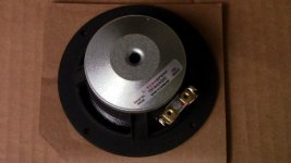
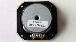
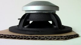
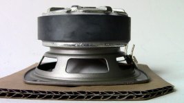
Magnets and mounting...
This is were the significant cost difference starts to reveal itself.
Both magnets are vented. TC9 is ferrite, and the 10F uses Neodymium. The 10F is a lot more stealth in this regards.
The fit and finish on both baskets is very well done. TC9 is poly based and the 10F is cast aluminium.
For mounting, the 10F is circular, and if I choose to build an array with this driver in the future, I would need to cut these to truncate them for closer driver spacing. The TC9 is already array-able.
 Also, I was very happy to discover that the bezel on the front of the TC9 is flat, under the foam gasket. So one DOES have the option to front mount these. Normal considerations do apply in regards to beveling the inside to allow the cone freer movement. And depending on one's building technique, insetting the TC9 for flush mounting can be a challenge, but as I plan on doing this via adding a hardwood mosaic to the outside of the cabinets, this will not be a problem for me - just have to cut over 120 curvy triangle wedges to fit in those gaps. I would have to do something similar with the 10F too.
This is were the significant cost difference starts to reveal itself.
Both magnets are vented.
TC9 is ferrite, and the 10F uses Neodymium. The 10F is a lot more stealth in this regards.The fit and finish on both baskets is very well done. TC9 is poly based and the 10F is cast aluminium.
For mounting, the 10F is circular, and if I choose to build an array with this driver in the future, I would need to cut these to truncate them for closer driver spacing.
The TC9 is already array-able. Also, I was very happy to discover that the bezel on the front of the TC9 is flat, under the foam gasket. So one DOES have the option to front mount these. Normal considerations do apply in regards to beveling the inside to allow the cone freer movement. And depending on one's building technique, insetting the TC9 for flush mounting can be a challenge, but as I plan on doing this via adding a hardwood mosaic to the outside of the cabinets, this will not be a problem for me - just have to cut over 120 curvy triangle wedges to fit in those gaps. I would have to do something similar with the 10F too. Attachments
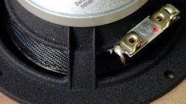
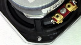
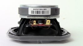
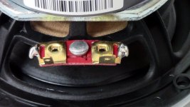
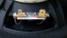
Terminals and profiles
The terminals are gold plated on both drivers, which is always a nice touch.
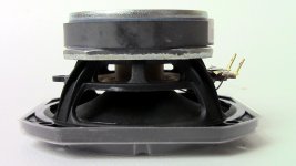
When looking at the side profile of these drivers, this is when You can see the amazing design work in the 10F, not that the TC9 is a slouch, because it is not. Yet, in theory, the 10F does allow a less obstructed back wave air flow. We will see over time, how well this works in practice. As I am considering the Fostex FF85 also, (last photo), You can see that the TC9 is more "stealth" compared to the FF85. So this is going to be interesting, as my adventure continues...
At some point, I will be comparing these drivers as point sources. When I get to that, I will link You to my thread.
Either way, I am building a TC9 array. Good thing too, because my "Cheap and Cheerfuls" are falling apart, so I need a "sensible" upgrade.
Allen
The terminals are gold plated on both drivers, which is always a nice touch.
When looking at the side profile of these drivers, this is when You can see the amazing design work in the 10F, not that the TC9 is a slouch, because it is not. Yet, in theory, the 10F does allow a less obstructed back wave air flow. We will see over time, how well this works in practice. As I am considering the Fostex FF85 also, (last photo), You can see that the TC9 is more "stealth" compared to the FF85. So this is going to be interesting, as my adventure continues...
At some point, I will be comparing these drivers as point sources. When I get to that, I will link You to my thread.
Either way, I am building a TC9 array. Good thing too, because my "Cheap and Cheerfuls" are falling apart
, so I need a "sensible" upgrade. Allen
Attachments
- Home
- Loudspeakers
- Full Range
- The making of: The Two Towers (a 25 driver Full Range line array)