Hi all
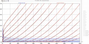
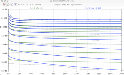
While playing with grid bias tube circuits, I realized that my Tungsol 12AX7 model is a bit off in terms of grid current below 100uA. This is because it used a Ig versus Vg chart (Va as parameter) but this was not a good choice - the traces are too close to each other, with the risk of misunderstandings.
However, I re-adjusted it for better accuracy.
Note the different suffix: .TSr4 (r=re-adjusted)
all the best, Adrian
Code:
*12AX7 LTspice model based on the generic triode model from Adrian Immler, version i4
*A version log is at the end of this file
*selection out of 5 new burnt-in Tung-Sol tubes and measurements done in May 2020
*Params re-adjusted to the measured values by Adrian Immler, March 2021
*The high fit quality is presented at adrianimmler.simplesite.com
*History's best of tube decribing art (plus some new ideas) is merged to this new approach.
*@ neg. Vg, Ia accuracy is similar to Koren or Ayumi models.
*@ small neg. Vg, the "Anlauf" current is considered.
*@ pos. Vg, Ig and Ia accuracy is on a unrivaled level.
*This offers new simulation possibilities like bias point setting with MOhm grid resistor,
*Audion radio circuits, low voltage amps, guitar distortion stages or pulsed stages.
*               re-adjusted TSi4 version (Ig model more accurate below 100uA)
*               |  anode (plate)
*               |  | grid
*               |  | | cathode
*               |  | | |
.subckt 12AX7.TSr4 A G K
+ params:
*Parameters for the space charge current @ Vg <= 0
+ mu   = 94.3  ;Determines the voltage gain @ constant Ia
+ rad  = 39k2  ;Differential anode resistance, set @ Iad and Vg=0V
+ Vct  = 0.28  ;Offsets the Ia-traces on the Va axis. Electrode material's contact potential
+ kp   = 950   ;Mimics the island effect
+ xs   = 1.5   ;Determines the curve of the Ia traces. Typically between 1.2 and 1.8
*
*Parameters for assigning the space charge current to Ia and Ig @ Vg > 0
+ kB   = 0.9   ;Describes how fast Ia drops to zero when Va approaches zero.
+ radl = 750   ;Differential resistance for the Ia emission limit @ very small Va and Vg > 0
+ tsh  = 12    ;Ia transmission sharpness from 1th to 2nd Ia area. Keep between 3 and 20. Start with 20.
+ xl   = 1.5   ;Exponent for the emission limit
*
*Parameters of the grid-cathode vacuum diode
+ kvdg  = 400  ;virtual vacuumdiode. Causes an Ia reduction @ Ig > 0.
+ kg = 6k      ;Inverse scaling factor for the Va independent part of Ig (caution - interacts with xg!)
+ Vctg = 0.23  ;Offsets the log Ig-traces on the Vg axis. Electrode material's contact potential
+ xg   = 1.65  ;Determines the curve of the Ig slope versus (positive) Vg and Va >> 0
+ VT   = 0.137 ;Log(Ig) slope @ Vg<0. VT=k/q*Tk (cathodes absolute temp, typically 1150K)
+ kVT=35m      ;Va dependant koeff. of VT
+ Vft2 = 1 gft2 = 20;finetunes the gridcurrent @ low Va and Vg near zero
*
*Parameters for the caps
+ cag  = 1p7   ;From datasheet
+ cak  = 0p34  ;From datasheet
+ cgk  = 1p6   ;From datasheet
*
*special purpose parameters
+ os = 1       ;Overall scaling factor, if a user wishes to simulate manufacturing tolerances
*
*Calculated parameters
+ Iad = {100/rad} ;Ia where the anode a.c. resistance is set according to rad.
+ ks = {pow(mu/(rad*xs*Iad**(1-1/xs)),-xs)} ;Reduces the unwished xs influence to the Ia slope
+ ksnom = {pow(mu/(rad*1.5*Iad**(1-1/1.5)),-1.5)} ;Sub-equation for calculating Vg0
+ Vg0 = {Vct + (Iad*ks)**(1/xs) - (Iad*ksnom)**(2/3)} ;Reduces the xs influence to Vct.
+ kl = {pow(1/(radl*xl*Ild**(1-1/xl)),-xl)} ;Reduces the xl influence to the Ia slope @ small Va
+ Ild = {sqrt(radl)*1m} ;Current where the Il a.c. resistance is set according to radl.
*
*Space charge current model
Bggi GGi 0 V=v(Gi,K)+Vg0 ;Effective internal grid voltage.
Bahc Ahc 0 V=uramp(v(A,K)) ;Anode voltage, hard cut to zero @ neg. value
Bst   St 0 V=uramp(max(v(GGi)+v(A,K)/(mu), v(A,K)/kp*ln(1+exp(kp*(1/mu+v(GGi)/(1+v(Ahc)))))));Steering volt.
Bs    Ai K I=os/ks*pow(v(St),xs) ;Langmuir-Childs law for the space charge current Is
*
*Anode current limit @ small Va
.func smin(z,y,k) {pow(pow(z+1f, -k)+pow(y+1f, -k), -1/k)} ;Min-function with smooth trans.
Ra  A Ai 1
Bgl Gi A I=min(i(Ra)-smin(1/kl*pow(v(Ahc),xl),i(Ra),tsh),i(Bgvd)*exp(4*v(G,K))) ;Ia emission limit
*
*Grid model
Bvdg G Gi I=1/kvdg*pwrs(v(G,Gi),1.5) ;Reduces the internal effective grid voltage when Ig rises
Rgip G Gi 1G ;avoids some warnings
Cvdg G Gi 0p1;this small cap improves convergence
.func fVT() {VT*exp(-kVT*sqrt(v(A,K)))}
.func Ivd(Vvd, kvd, xvd, VTvd)  {if(Vvd < 3, 1/kvd*pow(VTvd*xvd*ln(1+exp(Vvd/VTvd/xvd)),xvd), 1/kvd*pow(Vvd, xvd))} ;Vacuum diode function
Bgvd Gi K I=Ivd(v(G,K) + Vctg, kg/os, xg, fVT())
.func ft2() {gft2*(1-tanh(3*(v(G,K)+Vft2)))} ;Finetuning-func. improves ig-fit @ Vg near -0.5V, low Va.
Bgr Gi Ai I=ivd(v(GGi),ks/os, xs, 0.8*VT)/(1+ft2()+kB*v(Ahc));Is reflection to grid when Va approaches zero
Bs0 Ai K  I=ivd(v(GGi),ks/os, xs, 0.8*VT)/(1+ft2()) - os/ks*pow(v(GGi),xs) ;Compensates neg Ia @ small Va and Vg near zero
*
*Caps
C1 A G {cag}
C2 A K {cak}
C3 G K {cgk}
.ends
*
*Version log
*i1 :Initial version
*i2 :Pin order changed to the more common order A G K (Thanks to Markus Gyger for his tip)
*i3 :bugfix of the Ivd-function: now also usable for larger Vvd
*i4: Rgi replaced by a virtual vacuum diode (better convergence). ft1 deleted (no longer needed)
;2 new prarams for Ig finetuning @ Va and Vg near zero. New overall skaling factor os for aging etc.
Attachments
Wonderful friend, thank you very much.
This wave I can attack a hectode with this signal and build a simulation of a radio to lamps and make all the circuits.
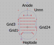
I find myself with a problem, the hectode I have of lts spice does not come with the triode, so in this type of lamps the cathode is common between the hectode and the triode, and the grid of the triode is internally linked to G1 of the hectode.
Do you think that this is any problem to make a simulation of a local oscillator and a mixture of the radio frequency signal with that of the local oscillator and directly attack the intermediate frequency transformers?
Thank you very much, if you made a simulation of a radio to lamps and share your file with me, I am very grateful.
This wave I can attack a hectode with this signal and build a simulation of a radio to lamps and make all the circuits.
I find myself with a problem, the hectode I have of lts spice does not come with the triode, so in this type of lamps the cathode is common between the hectode and the triode, and the grid of the triode is internally linked to G1 of the hectode.
Do you think that this is any problem to make a simulation of a local oscillator and a mixture of the radio frequency signal with that of the local oscillator and directly attack the intermediate frequency transformers?
Thank you very much, if you made a simulation of a radio to lamps and share your file with me, I am very grateful.
.SUBCKT HepthodeD 1 2 3 4 5; A G3 G2G4 G1 C
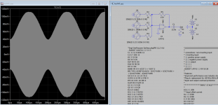
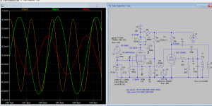
It's heptode, no triode model, you're correct, but triode mode can be separately built.
I'll try to sim the schematic as attached, see how it comes out.
It's heptode, no triode model, you're correct, but triode mode can be separately built.
I'll try to sim the schematic as attached, see how it comes out.
Attachments
Last edited:
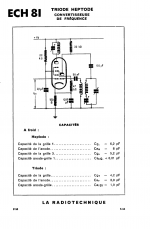
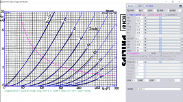
This is ECH81 triode model based on Philips, u=22.
Code:
* [url=http://www.dmitrynizh.com/tubeparams_image.htm]Model Paint Tools: Trace Tube Parameters over Plate Curves, Interactively[/url]
* Plate Curves image file: ech81-t.png
* Data source link:
*----------------------------------------------------------------------------------
.SUBCKT ECH81_T 1 2 3 ; Plate Grid Cathode
+ PARAMS: CCG=2.6P  CGP=1P CCP=2.1P
+ MU=22.22 KG1=1438.2 KP=59.15 KVB=1560 VCT=0.378 EX=1.428
+ VGOFF=-0.6 IGA=6.9E-4 IGB=0.156 IGC=4.88 IGEX=1.04
* Vp_MAX=300 Ip_MAX=20 Vg_step=2 Vg_start=0 Vg_count=9
* Rp=4000 Vg_ac=55 P_max=0.8 Vg_qui=-48 Vp_qui=300
* X_MIN=32 Y_MIN=60 X_SIZE=785 Y_SIZE=526 FSZ_X=1296 FSZ_Y=736 XYGrid=false
* showLoadLine=n showIp=y isDHT=n isPP=n isAsymPP=n showDissipLimit=y
* showIg1=y gridLevel2=y isInputSnapped=n
* XYProjections=n harmonicPlot=n dissipPlot=n
*----------------------------------------------------------------------------------
E1 7 0 VALUE={V(1,3)/KP*LOG(1+EXP(KP*(1/MU+(VCT+V(2,3))/SQRT(KVB+V(1,3)*V(1,3)))))}
RE1 7 0 1G  ; TO AVOID FLOATING NODES
G1 1 3 VALUE={(PWR(V(7),EX)+PWRS(V(7),EX))/KG1}
RCP 1 3 1G   ; TO AVOID FLOATING NODES
C1 2 3 {CCG} ; CATHODE-GRID
C2 2 1 {CGP} ; GRID=PLATE
C3 1 3 {CCP} ; CATHODE-PLATE
RE2 2 0 1G
EGC 8 0 VALUE={V(2,3)-VGOFF} ; POSITIVE GRID THRESHOLD
GG 2 3 VALUE={(IGA+IGB/(IGC+V(1,3)))*(MU/KG1)*(PWR(V(8),IGEX)+PWRS(V(8),IGEX))}
.ENDS
*$
Attachments
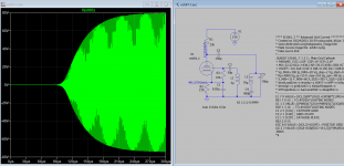
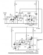
Project: Experimental Two Valve Superhet with no IF Amp.
This 2 valves superhet should be easier to sim and build.
This 2 valves superhet should be easier to sim and build.
Attachments
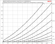
Hi - first time using the Dmitry Composite model tool. I am attempting to make a model for the 3C24 in A2 operation. The curves being matched to are real world curves from my curve tracer.

I have been able to get a reasonably good fit with the tool, shown above, however I am seeing an issue when implementing the model in circuit.
When operating in A2, the model hard clips at +50V on the grid and 150V on the plate, the grid current draw becomes excessive at that point, far higher than it should based on the model curves. On the +50V grid line, grid current should not sharply rise until close to plate saturation, around 75V on the plate. I turned off the advanced grid current option and used flat, constant grid current curves with the same result.
Any thoughts on why that would be? My circuit uses a direct-coupled cathode follower, although I see the same behavior using a FET source follower. Also, swapping to an 801 A2 model, created by Ale Moglia using the Dmitry tool, does not show the same issue, so all signs point to a flaw in the model.
I appreciate the help, below is the model generated by the tool.
WARNING, MODEL NOT VETTED BELOW, DO NOT USE!
**** 3C24 ** Composite DHT with Advanced Grid Current **************
* Created on 03/24/2021 14:27 using paint_kit.jar 3.1
* Model Paint Tools: Trace Tube Parameters over Plate Curves, Interactively
* Plate Curves image file: 3C24
* Data source link:
*----------------------------------------------------------------------------------
.SUBCKT DHT_3C24_A2 1 2 3 4 ; P G K1 K2
+ PARAMS: CCG=2.1P CGP=1.3P CCP=0.2P RFIL=2.1
+ MU=21.18 KG1=8874.87 KP=1500 KVB=473.1 VCT=0.2 EX=1.54
+ VGOFF=-1.5 IGA=0.0025 IGB=0.06358 IGC=-12 IGEX=1.841
* Vp_MAX=700 Ip_MAX=250 Vg_step=10 Vg_start=100 Vg_count=14
* Rp=4000 Vg_ac=55 P_max=25 Vg_qui=-48 Vp_qui=300
* X_MIN=131 Y_MIN=20 X_SIZE=548 Y_SIZE=534 FSZ_X=1260 FSZ_Y=630 XYGrid=false
* showLoadLine=n showIp=y isDHT=y isPP=n isAsymPP=n showDissipLimit=y
* showIg1=y gridLevel2=y isInputSnapped=n
* XYProjections=n harmonicPlot=n dissipPlot=n
*----------------------------------------------------------------------------------
RFIL_LEFT 3 31 {RFIL/4}
RFIL_RIGHT 4 41 {RFIL/4}
RFIL_MIDDLE1 31 34 {RFIL/4}
RFIL_MIDDLE2 34 41 {RFIL/4}
E11 32 0 VALUE={V(1,31)/KP*LOG(1+EXP(KP*(1/MU+V(2,31)/SQRT(KVB+V(1,31)*V(1,31)))))}
E12 42 0 VALUE={V(1,41)/KP*LOG(1+EXP(KP*(1/MU+V(2,41)/SQRT(KVB+V(1,41)*V(1,41)))))}
RE11 34 0 1G
G11 1 31 VALUE={(PWR(V(32),EX)+PWRS(V(32),EX))/(2*KG1)}
G12 1 41 VALUE={(PWR(V(42),EX)+PWRS(V(42),EX))/(2*KG1)}
RCP1 1 34 1G
C1 2 34 {CCG} ; CATHODE-GRID
C2 2 1 {CGP} ; GRID=PLATE
C3 1 34 {CCP} ; CATHODE-PLATE
RE2 2 0 1G
EGC1 81 0 VALUE={V(2,31)-VGOFF} ; POSITIVE GRID THRESHOLD
GG1 2 31 VALUE={0.5*(IGA+IGB/(IGC+V(1,31)))*(MU/KG1)*(PWR(V(81),IGEX)+PWRS(V(81),IGEX))}
EGC2 82 0 VALUE={V(2,41)-VGOFF} ; POSITIVE GRID THRESHOLD
GG2 2 41 VALUE={0.5*(IGA+IGB/(IGC+V(1,41)))*(MU/KG1)*(PWR(V(82),IGEX)+PWRS(V(82),IGEX))}
.ENDS
*$
Koonw friend, I am very grateful, but opening this file throws me this lt spice problem.
Do i need hectode lt spice model complete with pentode and triode. Can you provide this to me to solve the problem?
Thank you very much friend, have a good day.
erwerwerw — ImgBB
Captura — ImgBB


Do i need hectode lt spice model complete with pentode and triode. Can you provide this to me to solve the problem?
Thank you very much friend, have a good day.
erwerwerw — ImgBB
Captura — ImgBB
Last edited:
Vacuum Tube SPICE Models
Vacuum Tube SPICE Models
You need both models. You can paste the model using spice directive or save the file in lib directory, and use ".inc ech81.inc" statement or UN-comment the statement if you don;t save it as a file.,
Vacuum Tube SPICE Models
You need both models. You can paste the model using spice directive or save the file in lib directory, and use ".inc ech81.inc" statement or UN-comment the statement if you don;t save it as a file.,
For the sake of closing the loop on my last post, my 3C24 model is now working as intended. Dmitry Nizh helped troubleshoot the issue, related to the high value of KP which does not sit well with LTSpice math.
Here is the completed model and curve overlay.

Here is the completed model and curve overlay.
**** 3C24 ** Composite DHT with Advanced Grid Current **************
* Created on 03/28/2021 07:38 using paint_kit.jar 3.1
* Model Paint Tools: Trace Tube Parameters over Plate Curves, Interactively
* Plate Curves image file:
* Data source link:
*----------------------------------------------------------------------------------
.SUBCKT DHT_3C24_A2 1 2 3 4 ; P G K1 K2
+ PARAMS: CCG=2.1P CGP=1.3P CCP=2.1P RFIL=2.1
+ MU=21.18 KG1=8874.87 KP=150 KVB=473.1 VCT=0.2 EX=1.54
+ VGOFF=-1.5 IGA=0.0025 IGB=0.06358 IGC=-12 IGEX=1.841
* Vp_MAX=700 Ip_MAX=250 Vg_step=10 Vg_start=100 Vg_count=14
* Rp=4000 Vg_ac=55 P_max=25 Vg_qui=-48 Vp_qui=300
* X_MIN=203 Y_MIN=30 X_SIZE=453 Y_SIZE=442 FSZ_X=1260 FSZ_Y=630 XYGrid=false
* showLoadLine=n showIp=y isDHT=y isPP=n isAsymPP=n showDissipLimit=y
* showIg1=y gridLevel2=y isInputSnapped=n
* XYProjections=n harmonicPlot=n dissipPlot=n
*----------------------------------------------------------------------------------
RFIL_LEFT 3 31 {RFIL/4}
RFIL_RIGHT 4 41 {RFIL/4}
RFIL_MIDDLE1 31 34 {RFIL/4}
RFIL_MIDDLE2 34 41 {RFIL/4}
E11 32 0 VALUE={V(1,31)/KP*LOG(1+EXP(KP*(1/MU+V(2,31)/SQRT(KVB+V(1,31)*V(1,31)))))}
E12 42 0 VALUE={V(1,41)/KP*LOG(1+EXP(KP*(1/MU+V(2,41)/SQRT(KVB+V(1,41)*V(1,41)))))}
RE11 34 0 1G
G11 1 31 VALUE={(PWR(V(32),EX)+PWRS(V(32),EX))/(2*KG1)}
G12 1 41 VALUE={(PWR(V(42),EX)+PWRS(V(42),EX))/(2*KG1)}
RCP1 1 34 1G
C1 2 34 {CCG} ; CATHODE-GRID
C2 2 1 {CGP} ; GRID=PLATE
C3 1 34 {CCP} ; CATHODE-PLATE
RE2 2 0 1G
EGC1 81 0 VALUE={V(2,31)-VGOFF} ; POSITIVE GRID THRESHOLD
GG1 2 31 VALUE={0.5*(IGA+IGB/(IGC+V(1,31)))*(MU/KG1)*(PWR(V(81),IGEX)+PWRS(V(81),IGEX))}
EGC2 82 0 VALUE={V(2,41)-VGOFF} ; POSITIVE GRID THRESHOLD
GG2 2 41 VALUE={0.5*(IGA+IGB/(IGC+V(1,41)))*(MU/KG1)*(PWR(V(82),IGEX)+PWRS(V(82),IGEX))}
.ENDS
*$
6N27P spice model
I have this one that I made in Curve Captor.Has anybody got a reliable spice model
for ECC86 or 6GM8 or 6N27P ??
Code:
* ==============================================================
* 6N27P LTSpice model
* Vp max=30V
* Rydel model (5 parameters): mean fit error 0.0929598mA
* Traced by Wayne Clay on 02/20/2019  using Engauge Digitizer 10.4
* and Curve Captor v0.9.1 from Soviet data sheet.
* ==============================================================
.subckt 6N27P  P G K
    Bp  P K  I=
+ ((0.06761422227m)+(0.02514297819m)*V(G,K))*uramp((10.49851918)*V(G,K)+
+ V(P,K)+(3.457647953))**1.5 * V(P,K)/(V(P,K)+(0.1934578768))
    Cgp G P 2.0p ; 0.7p added (1.3p)
    Cgk G K 3.7p ; 0.7p added (3.0p)
    Cpk P K 0.4p ; 0.2p added (0.2p)
    Cps P 0 1.6p ; Plate to shield (shield connected to ground)
    Rpk P K 1.0G ; to avoid floating nodes
    d3  G K dx1
.model dx1 d(is=1n rs=2k cjo=1pf N=1.5 tt=1n)
.ends 6N27P
Attachments
- Home
- Amplifiers
- Tubes / Valves
- Vacuum Tube SPICE Models