Hi David, I would to ask does hornresp have Mac version? Kind Regards,
Hi Everyone,
CHANGE
When the construction data for a Le Cléac'h horn is exported it is possible to specify either the standard 2007 flare profile (which becomes slightly inaccurate near the horn mouth) or the exact axisymmetric profile.
Previously when the Exact Profile option was selected it was possible to choose from either the Axisymmetric Horn, Rectangular Horn or Petal Horn options, even though only the axisymmetric profile data would be exported, regardless of the option chosen. Attachment 1 refers.
Now when the Exact Profile option is selected, the Rectangular Horn and Petal Horn options are hidden to avoid any confusion. Attachment 2 refers.
(The axisymmetric, rectangular and petal horn data export options are all still available when the Standard Profile option is selected. Attachment 3 refers).
Kind regards,
David
hornresp doesn´t run on MAC OS (X).
You can use something like
vmware Fusion (virtualization)
boot camp (install windows on your mac)
Parralels Desktop (virtualization)
Virtual Box (virtualization)
Wine (came from the linux world and lets you run many windows apps, on OSX, take a look at crossover, which uses the same base but is more user friendly)
hornresp also runs on Reactos (windows re-done from scratch for free)
If you need help with this, please don´t hesitate to ask
Constant diaphragm velocity:
1/2 displacement per octave frequency increase
1/10 displacement per decade frequency increase
Constant diaphragm acceleration:
1/100 displacement per decade frequency increase
For the sake of completeness...
Constant diaphragm acceleration:
1/4 displacement per octave frequency increase
That's a good thing tho'! Thank you again David for such a wonderful program!
Thanks BP1Fanatic.
Thanks BP1Fanatic.
You're welcome guy!
Constant diaphragm acceleration vs velocity
Hi David,
I still don't understand, why constant velocity drive of the diaphragm is preferred over constant acceleration drive.
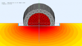
I did a short series of simulations in ABEC comparing constant velocity drive vs constant acceleration vs LEM / TSP drive of the same 2''-diaphragm in a very simple enclosure:

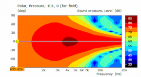
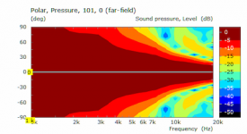
Directivity for the membrane driven with the TSP taken from a 2'' TangBand chassis (W2-748SG):
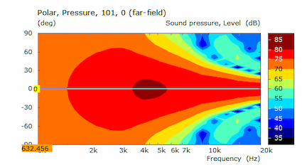
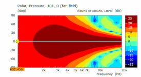
Same membrane in same enclosure, driven by constant acceleration:

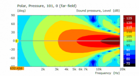
Same membrane, same enclosure, membrane driven by constant velocity:
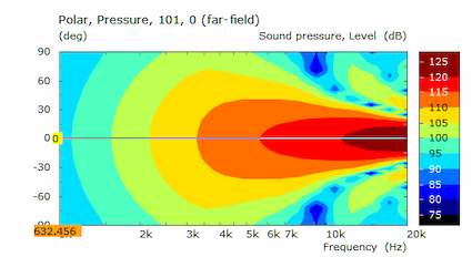
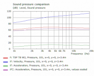
Comparison of SPL on axis in one image (TSP-driven, const. acceleration, const. velocity):
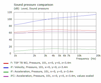
Not very surprising, this shows the SPL increase with increasing frequency for constant velocity. It shoes as well the very similar SPL for constant acceleration and TSP-drive of the membrane.
Of course, as long as we look at normalized directivity of a horn, it does not matter, which type of drive is applied to the membrane (see control-check, i.e. normalized directivity). This is identical for all three types of drive:

As constant acceleration reflects SPL of a driver much better than constant velocity drive - why is constant velocity drive still preferred for HornResp simulation? Does this fit better to compression driver behaviour (I did not look at this, but DonVKs comment suggest this)? I may have missed something here though...
PS: Discussed here before...
Hi David,
Quote:
Originally Posted by DonVK View Post
There was also some discussion around that time regarding constant acceleration as well. Do you know why or where constant acceleration would be useful in modelling?
Hi Don,
I was never quite sure how Jean-Michel intended using results generated by a constant diaphragm acceleration model. Tragically he is no longer with us to clarify what he had in mind. The theory involved is simple enough, though.
////////////////////////////////////////////
Given:
w = 2 * Pi * f
Da = constant diaphragm acceleration
Dd = diaphragm displacement
Then:
Dd = Da / (w ^ 2)
////////////////////////////////////////////
Kind regards,
David
I still don't understand, why constant velocity drive of the diaphragm is preferred over constant acceleration drive.
I did a short series of simulations in ABEC comparing constant velocity drive vs constant acceleration vs LEM / TSP drive of the same 2''-diaphragm in a very simple enclosure:
Directivity for the membrane driven with the TSP taken from a 2'' TangBand chassis (W2-748SG):
Same membrane in same enclosure, driven by constant acceleration:
Same membrane, same enclosure, membrane driven by constant velocity:
Comparison of SPL on axis in one image (TSP-driven, const. acceleration, const. velocity):
Not very surprising, this shows the SPL increase with increasing frequency for constant velocity. It shoes as well the very similar SPL for constant acceleration and TSP-drive of the membrane.
Of course, as long as we look at normalized directivity of a horn, it does not matter, which type of drive is applied to the membrane (see control-check, i.e. normalized directivity). This is identical for all three types of drive:
As constant acceleration reflects SPL of a driver much better than constant velocity drive - why is constant velocity drive still preferred for HornResp simulation? Does this fit better to compression driver behaviour (I did not look at this, but DonVKs comment suggest this)? I may have missed something here though...
PS: Discussed here before...
Attachments
-
 2019-04-02 2-Zoll Membr in Enclosure Image 1.png111.6 KB · Views: 363
 -
 2019-04-02 2-Zoll Membr in Enclosure TSP TB W2 direct 1.png68 KB · Views: 327
 -
 2019-04-02 2-Zoll Membr in Enclosure Acceleration Drive direct 1.png66.2 KB · Views: 351
 -
 2019-04-02 2-Zoll Membr in Enclosure Velocity Drive direct 1.png73.6 KB · Views: 331
 -
 2019-04-02 2-Zoll Membr in Encl Velocity-Accel-LEM_TSP SPL 1.png72.1 KB · Views: 335
 -
 2019-04-02 2-Zoll Membr in Enclosure TSP TB W2 direct norm0 1.png65.7 KB · Views: 357
Last edited:
As constant acceleration reflects SPL of a driver much better than constant velocity drive - why is constant velocity drive still preferred for HornResp simulation?
Hi Gaga,
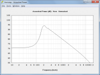
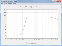
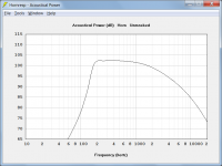
The three attachments show the power response of a 160Hz Le Cléac'h horn with T = 0.8, under the following conditions:
Attachment 1 - TAD TD2001 driver with Eg = 2.83 volts rms
Attachment 2 - Driver diaphragm with a constant velocity of 10 cm/sec rms
Attachment 3 - Driver diaphragm with a constant acceleration of 100 m/sec2 rms
As you can see, the constant acceleration result is very different to the constant voltage and constant velocity results.
The constant velocity option was requested by Jean-Michel, who is sadly no longer with us. The following comments in quotes are taken from two of his posts:
"The constant velocity diaphragm will be very useful to compare horns without the influence of the driver."
"You can simulate a 1" or a 2" horn without knowing the Thiele and Small parameters, introducing Eg = 0 (in place of the normal value Eg = 2,83). Doing this the driver will be considered as a "constant velocity source". This feature is very interesting when designing new horns without knowing the Thiele and Small parameters. For sure the results will be better than with a real driver, specially in the HF (because moving mass = 0)."
Jean-Michel was also the first person to mention constant acceleration, but the option was not added to Hornresp because he didn't specifically request that it be included.
Kind regards,
David
Attachments
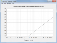
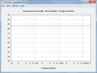
Further to my post above, note the on-axis pressure results when constant velocity and constant acceleration are applied to a piston in an infinite baffle.
Attachment 1 - Constant piston velocity of 10 cm/sec rms
Attachment 2 - Constant piston acceleration of 100 m/sec2 rms
(Sd = 150 cm2 in each case).
Attachment 1 - Constant piston velocity of 10 cm/sec rms
Attachment 2 - Constant piston acceleration of 100 m/sec2 rms
(Sd = 150 cm2 in each case).
Attachments
Hi David,
I did some experiments similar to what you mentioned. I was comparing HornResp to ABEC models. I tried this for 3 compression drivers and 2 horns and the results [compression driver, velocity, acceleration] were similar to what you posted.
If we use constant velocity. It appears to model the CD better in the frequency region around horn cutoff and where the impedance is changing. However its not accurate at predicting the attenuation at higher freq. HornResp predicts a output rising faster than ABEC but the issue is still there.
If we use constant acceleration. It appears to model the CD better in the frequency region where the impedance is more constant and the output starts dropping off. However, it's not accurate at predicting the output around cutoff.
It seems that we also need the regions where the "constant" assumption applies.
Hi David, hi Don,
Thanks a lot for your replies.
From my point of view, constant acceleration could be used to evaluate horn characteristics independently of driver characteristics as well.
However, I'm a bit surprised about the behavior of the compression driver models. I could not find any TSP for the TAD TD2001. Would you mind to post the TSP values you used to model a compression driver in HornResp? Would appreciate very much...
Kind regards,
Christoph
Thanks a lot for your replies.
Yes, I think we agree, that constant velocity drive significantly overestimates SPL at high frequencies. May be this behaviour (masking the 'natural' roll-off towards high frequencies by constant velocity drive) was suggested to be helpful to evaluate horns by JMLC."You can simulate a 1" or a 2" horn without knowing the Thiele and Small parameters, introducing Eg = 0 (in place of the normal value Eg = 2,83). Doing this the driver will be considered as a "constant velocity source". This feature is very interesting when designing new horns without knowing the Thiele and Small parameters. For sure the results will be better than with a real driver, specially in the HF (because moving mass = 0)."
From my point of view, constant acceleration could be used to evaluate horn characteristics independently of driver characteristics as well.
However, I'm a bit surprised about the behavior of the compression driver models. I could not find any TSP for the TAD TD2001. Would you mind to post the TSP values you used to model a compression driver in HornResp? Would appreciate very much...
Kind regards,
Christoph
There is a TD2001 driver at High Efficiency Speaker Asylum: Hornresp and TD2001 simulation by Jmmlc
David may be using a different one.
The thread Modelling compression drivers has some more.
David may be using a different one.
The thread Modelling compression drivers has some more.
Last edited:
Hi David.
I think there is no doubt that spl is proportional to acceleration of the diaphragm. Therefore with constant velocity we cannot simulate the falling response of a compression driver in a horn within its normal operating range. For constant velocity acceleration is zero and this cannot be true. Maybe it is valid to Show the properties of the Horn itself.
The cycle time for low freqs is largeer and with constant velocity the diaphragm receives a higher velocity and more spl. I assume that JMLC was interested in the constant accl feature because he intended to get a rough impression how an ideal driver would show up the generally observed falling spl towards higher freqs
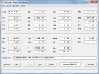
I could not find any TSP for the TAD TD2001. Would you mind to post the TSP values you used to model a compression driver in HornResp?
Hi Christoph,
I used the values shown in the attachment.
(The driver and chamber values are the same as those given by Don in his first linked post).
Kind regards,
David
Attachments
For constant velocity acceleration is zero
Hi docali,
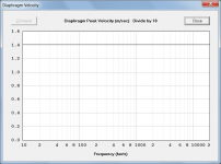
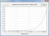
The term constant velocity as used in Hornresp means that the rms and peak values of the diaphragm velocity do not change with frequency. The actual velocity and acceleration of the diaphragm will vary sinusoidally with a 90 degree phase difference between the two.
For constant peak velocity as shown in Attachment 1, the peak acceleration varies as shown in Attachment 2.
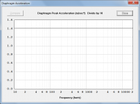
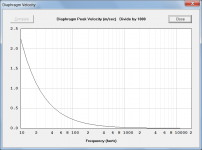
For constant peak acceleration as shown in Attachment 3, the peak velocity varies as shown in Attachment 4.
Kind regards,
David
Attachments
Hi David,
Would you consider adding constant acceleration drive. Maybe via further overloading on the Eg variable?
Eg > 0 : actual drive voltage
Eg = 0 : constant velocity 0.1m/s
Eg < 0 : constant acceleration 100m/s
P.S. The constant acceleration graph appears to already be in hornresp. Is that a special build or foresight") ?
?
many thanks
Don
Would you consider adding constant acceleration drive. Maybe via further overloading on the Eg variable?
Eg > 0 : actual drive voltage
Eg = 0 : constant velocity 0.1m/s
Eg < 0 : constant acceleration 100m/s
P.S. The constant acceleration graph appears to already be in hornresp. Is that a special build or foresight
?many thanks
Don
Last edited:
Hi David,
Of course, as long as we look at normalized directivity of a horn, it does not matter, which type of drive is applied to the membrane (see control-check, i.e. normalized directivity). This is identical for all three types of drive:
Of course, since unless the driving method can change how the diaphragm breaks up, it cannot change the directivity. Which again highlights the fact that you cannot modify the directivity of a single driver by electronic means.
As constant acceleration reflects SPL of a driver much better than constant velocity drive - why is constant velocity drive still preferred for HornResp simulation?
Constant acceleration gives flat SPL for a direct radiator, where the radiation resistance increases 12dB/octave. This is not the case for horns.
- Home
- Loudspeakers
- Subwoofers
- Hornresp