Hello,
i need to make a Boost PFC inductor. (Its for a CCM PFC stage which will be follwed by a 330W, split output, 2 transistor forward converter for Class B amp supply.)
Inductor spec:
L = 331uH
I(RMS) = 5A2
I(PK) = 9A7
Switching frequency = 60KHz.
Do you know of any good families of ferrite cores that i can use to wind this?
A the moment i am intending to use the ETD 54 core with 2mm gap as follows....
http://www.epcos.com/inf/80/db/fer_07/etd_54_28_19.pdf
I intend to use 38 turns to get 331uH , however, i am worried about the openness of the core, and how it may interfere with other circuitry via its fields, and also the 2mm air gap in the centre post may overheat the windings near to it?
core loss can be calculated by flux swing, and is mateeial dependant. as frequency is quote.low i would look into material sutable for 100+ kHz operation.
Perhaps you could.look into the better iron alloy materials like Sendust , a distributed gap gives less fringing losses around the.gap as these are.hard to calculate.
check out.powermagnetics (pace) webpage, they.are UK bbased and sell to EU for privateers")
Perhaps you could.look into the better iron alloy materials like Sendust , a distributed gap gives less fringing losses around the.gap as these are.hard to calculate.
check out.powermagnetics (pace) webpage, they.are UK bbased and sell to EU for privateers
Hi,
Thanks but PQ cores, made by Ferroxcube and Epcos, do not come with gaps, so they will saturate at the current levels that i am using.
I would need to add a gap of 1.2mm to the PQ5050 core and this would mean the fringing field being significant and the usual reluctance method wont work to calculate the new inductance of the turns on the gapped core.....3D magnetic simulation is reguired and it costs $1000's.
i cannot understand why gapped cores of big ferrite cores are not available?
i think you are up for some experiment then, testing the core to see the heating effect of the.losses.
as for larger pq cores with an huge air gap- why would they manufacture these? one major pro for the pq core is the better shielding (but con is worse cooling) and the shielding effect is reduced by the gappin'
perhaps you can shims the core and put a flux band. still need to test for losses though. dont waste money on a simulation, spend it on testing instead. then you will know.
Treez, for a center-leg gap, you'll have to either gap the core yourself, or send it to someone to get gapped.
For an ETD54, if you pick a ferrite with a decent high-temperature saturation flux density like say 3C96, and choose Bmax = 300mT you will need a 2.4mm gap and 38 turns.
If you use a PQ5050, you will need a 1.8mm gap and 33 turns.
all calculated
I have transcribed the entire ferroxcube databook into Mathcad, along with lots of data on core materials etc. and spent a long time working out how to design all this stuff numerically - including variation of Bsat with temp etc. all fun and games. Its handy to be able to create ones own Hanna curves - I invariably find the ferroxcube databook hasn't got a Hanna curve for the core I'm using. Grrrr
Last edited:
Another vote for toroid Sendust (aka kool-mu or super-mss). Less field and way more forgiving on saturation.
Like this one maybe:
http://www.feryster.com.pl/polski/pdf/dlawiki/DTMSS-40_0,33_8,0.pdf
Like this one maybe:
http://www.feryster.com.pl/polski/pdf/dlawiki/DTMSS-40_0,33_8,0.pdf
I dont think that leakage flux is avoidable, the air .must get in there either localized (air gap) or .distributed.
question is which is worst?
A centre gap , covered with winding and perhaps a. flux band OR a powder core , covered with winding around the radius with a flux band ?
I dont know , I am just an amateur I guess that is what experience is for
question is which is worst?
A centre gap , covered with winding and perhaps a. flux band OR a powder core , covered with winding around the radius with a flux band ?
I dont know , I am just an amateur
I guess that is what experience is for I dont think that leakage flux is avoidable, the air .must get in there either localized (air gap) or .distributed.
question is which is worst?
A centre gap , covered with winding and perhaps a. flux band OR a powder core , covered with winding around the radius with a flux band ?
I dont know , I am just an amateur
sorry, that came across wrong - prose fail. you're quite right. FWIW I figured you weren't an amateur.....
there really isnt a "best" - it depends entirely on what you're trying to achieve and why, and what you can actually get. every approach is bad if done wrong, and if done right they are all pretty good.
about the only hard and fast rule I have is this: never, ever use bobbin cores. they have the air gap on the outside..... the shielded ones arent too bad (but not as good as your suggestions), but unshielded is a nightmare.
and make sure you take skin and more importantly proximity effect into account.
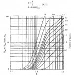
Ahem. I got a bit carried away, and generated the attached graph for DIYAudio. Its a plot of AC-to-DC resistance ratio Fr, versus phi, which is the ratio of equivalent wire thickness (usually given the greek symbol Phi) to skin depth, for varying numbers of effective layers (usually called "p").
If you interleave your windings (eg 1/2P,S,1/2P) there is a line of symmetry through the center of the secondary - the windings "look" the same above and below this line. the number of effective layers in each winding is now HALF of the actual no. of layers.
eg we have a 4-layer primary with a 1-layer secondary on top. p_pri = 4, p_sec = 1
but if we interleave it then we get p_pri = 2, p_sec = 0.5
Phi is a horrible function of bare and insulated wire diameter, bobbin winding width, core center-leg length and turns-per-layer. I did some re-arranging, and came up with a really simple approximation thats good for wire with thin insulation. it takes into account all the packing factors (averaged across entire families of core/bobbin sets) and only needs wire diameter and switching frequency. MKS units, so m & Hz. And I inverted the approximation, so you can pick some Fr, find Phi then calculate wire diameter.
to see the advantage of interleaving, use the above p-values, with Phi = 2.
non-interleaved:
Fr_pri = 18 so Rac_pri = 18*Rdc_pri
Fr_sec = 1.9 so Rac_sec = 1.9*Rdc_sec
interleaved:
Fr_pri = 5.1 so Rac_pri = 5.1*Rdc_pri
Fr_sec = 1.1 so Rac_sec = 1.1*Rdc_sec
the primary Ac copper loss went down threefold!
the advantage of a gap, center-leg or core separation, is that the gap and hence fringing field is in a known & controlled place. so you can put a belly band on it to shield it, and not point it at something sensitive. center leg gaps are the best, but you do need to be careful of excess losses in the winding.
belly bands almost always help. in say an etd core, most of the winding is hanging out in free space - good for cooling and leaking flux. wind a planar xfmr on say an EI22, and half the damn winding is hanging out. Pot cores solve that problem, and replace it with thermal and "where do the wires come out" problems. PQ's are a compromise, giving quite a lot of core coverage but with a decent chunk exposed for cooling and leadouts. and its pretty easy to cover the big holes with a fat belly band.
One approach to avoid fringing flux related copper loss but that makes the winding look ugly and wastes a chunk of the winding area is to make a "lump" in the bobbin around the center, to lift the winding away from the gap. if the lump holds the winding a couple of gap lengths further out, and extends a couple of gap lengths either side of the gap, it can make a noticeable difference. litz is good too, if you can get it.
the distributed airgap cores have less problem with excess copper loss as the amount of fringing flux in any one place is a lot less - because its leaking a bit everywhere. And if you have a large AC component core loss will be a problem - and the less lossy a material is, the lower its permeability (generalising). so as you try to reduce core loss, you end up spraying flux everywhere (and coupling to any other cores doing likewise). I found that out the hard way, trying to reduce core loss by using -2 material.
the koolmu type cores are pretty good for losses (ferrites still win, with room to spare) but wow. $$$ even in volume. like 10x the cost of a -52 core the same size. funny thing is, thats probably much less of a problem for DIY stuff (assuming you can actually get them), and being able to buy a bag of 500 -52 cores for like 20c each is probably equally unappealing. I havent looked for a few years, and based on this thread its pretty clear there's a bunch of materials to look at. thanks
When there is a big DC component (so the AC core losses are small) iron powder is great. one sneaky gotcha is that the permeability drops off with frequency - and when it gets to one, its air cored. but thats at the MHz or so mark, eg I use -52 material over say -26 for that reason (it plays hell with many an EMI filter).
toroids are a pain to wind, especially with big fat wires. sore fingers.
to be honest the method I learned was "only choose cores you can actually get". by picking a core, then having the xfmr manufacturer or core vendor say things like MOQ 50,000 pieces, 26 weeks delivery. repeatedly.
Attachments
Another vote for toroid Sendust (aka kool-mu or super-mss). Less field and way more forgiving on saturation.
Like this one maybe:
http://www.feryster.com.pl/polski/pdf/dlawiki/DTMSS-40_0,33_8,0.pdf
To address questions: 75 init perm sendust, ~7USD for a ready choke, ~2USD for a bare core where I live
Terry, reading (and understanding) posts like yours reduces my amateurism
Thanks for the effort with the attachment, basically a Dowell curve if I understand it correct.That goes to everybody how posts here actually. Thank you!
Good tip about the "put some distance between winding and gap" to reduce losses.
I started played with iron powder cores (bad old -26 material , ripped out of old computer power supplies) a lot with buck converters and then the falling permeability(due to Oersteds, not Hertz) is not so much of a problem, yes- current ripple increases with increasing current due to this but usually not so much that the converter falls into discontinous mode and you need to have some margin in the output capacitors anyhow for ripple current capacity (besides it is the input caps that really takes a beating ..)
Advantage of beeing a hobbyist is just as you point out, budget restraints are not so hard. Fex ordering a reel of TIW is not completely unheard of solving some headaches like insulation ... (when applicable of course)
To be on topic-a PFC is designed with quite some ripple current and therefore high AC flux, and this causes losses in powder cores => necessary with enormous cores (to get lower flux) or more expensive material (still to much loss perhaps) or a combination.
It is hard to tell, you have to check out any material itself. And a good advice is look into avalibility. We have no clue about volumes.
But as Treez is UK (by the flag), check out Pace | Magnetics or feryster.com, the later I have no experience with myself.
Thanks for the effort with the attachment, basically a Dowell curve if I understand it correct.That goes to everybody how posts here actually. Thank you!
Good tip about the "put some distance between winding and gap" to reduce losses.
I started played with iron powder cores (bad old -26 material , ripped out of old computer power supplies) a lot with buck converters and then the falling permeability(due to Oersteds, not Hertz) is not so much of a problem, yes- current ripple increases with increasing current due to this but usually not so much that the converter falls into discontinous mode and you need to have some margin in the output capacitors anyhow for ripple current capacity (besides it is the input caps that really takes a beating ..)
Advantage of beeing a hobbyist is just as you point out, budget restraints are not so hard. Fex ordering a reel of TIW is not completely unheard of
solving some headaches like insulation ... (when applicable of course) To be on topic-a PFC is designed with quite some ripple current and therefore high AC flux, and this causes losses in powder cores => necessary with enormous cores (to get lower flux) or more expensive material (still to much loss perhaps) or a combination.
It is hard to tell, you have to check out any material itself. And a good advice is look into avalibility. We have no clue about volumes.
But as Treez is UK (by the flag), check out Pace | Magnetics or feryster.com, the later I have no experience with myself.
Rikkitikkitavi,
yep, thats it - Dowells curves. These are often done in an awkward, unhelpful manner - eg in Keith Billings book, where the vertical axis is not Fr, but an unhelpful intermediary step. Snelling kindly produces the Fr graph (which I have duplicated), but you'd better be sitting down when you try and purchase his book. my copy cost NZ$450, in 1994.
I realised after I'd posted it that I could have made another graph, using my simplified formula for Phi(od_Cu), and making the x-axis od_Cu/sqrt(f). the disadvantage of that is the resultant curves incorporate the wire, core and bobbin assumptions I used, whereas my original graph is exact.
it took me a while to reproduce Snellings graph though - lots of published papers have mistakes, and that really doesnt help - the paper by Petkov, although very good, has a garbled wreck in lieu of the actual Fr(Phi,p) equation.
just to complicate it further, there are lots of trigonometric equalities that can be used to express Fr(Phi) in elleventy different forms - that look entirely different. in addition to graphing several different formulae, I did the algebra to prove they were the same.
I also looked at some of the approximations for Fr(Phi,p). and they suck, badly. I've attached the graphs. The first approximation is OK for Phi < 2 - which is where you should be designing. the second approximation is only valid for Phi > 2 - it accurately represents the region where proximity effect has done its worst.
I'll explain that better: in the actual Fr(Phi,p) graph, each curve has three slopes. it starts out almost flat - no proximity effect at all. then it transitions too a steep slope. This is proximity effect, and the steep slope is why a moderate increase in wire size can lead to a massive increase in Fr. Years ago I fixed a 400:24V PFC transformer that set itself on fire - by reducing the foil thickness from 0.6mm to 0.1mm. I had a shouting match with the factory manager, who didn't believe me. In the end I got him to agree to try it, and if I were wrong I'd do something humiliating and public. final temperature rise ~25C (it was ~300C). He bought my drinks that night.
Eventually the slope of each curve reduces to a constant value. have a look, in this region if you double od_Cu and hence Phi, Fr doubles. but Rdc halves, so no net increase. and now look at the curves for p = 0.5 & 1 layer - there is no steep slope. so a single layer winding (or a two-layer winding in an interleaved design) is essentially immune to proximity effect. There is an optimum, but it only saves 8% or so. that means you can use thick-n-chunky wire to reduce thermal resistance, without incurring any real penalty (for high performance designs, 8% is worth having).
so that second approximation is utterly useless - it only works once proximity effect has done its worst. F***ing maths, how does that work?
plus once you have the graph of the real thing, who needs an approximation?
I can show my working if anyone is really interested.
Attachments
Terry, a short answer:
please do show your findings, understanding the Dowell curves and proximity effect is amongst the harder stuff in SMPS design, and also highly important, I would say more so than understanding skin effect when it comes to impact on performance.
regards
Rickard
please do show your findings, understanding the Dowell curves and proximity effect is amongst the harder stuff in SMPS design, and also highly important, I would say more so than understanding skin effect when it comes to impact on performance.
regards
Rickard
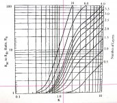
Terry Given, This is an official request for modification to your first chart. I have been looking for a colored chart to make reading of the Dowell curves easer. I have a black and white chart that is a nice one except no color, making it hard to pick out layers. And i wish the chart went up to 12 layers. If you would be so kind as to mod your chart here is my list of mods.
1) Add the words Rac/Rdc Ratio to vertical graph. See attached chart.
2) If possible label each layer on the end of the line on right side of chart and remove all of your text about FRH and layer color on the left side of chart. If you can not label each line with the layer number, then move the FRH text to the right side and reverse the order so it matches the graph. You have .5 layer on the top and 10 layers on the bottom. And for less confusion replace the comma after phi with a dash.
3) Add layers up to 12. I find i need this frequently. Please keep your layer numbers of 5, 6, 8, 10 and add 12. I like your jumping of two layers, not like my existing chart were it jumps 4 layers at the end. If the chart does not get to cluttered can you see what up to 20, or even 30 layers looks like ( bigger jumps on the end, maybe 4 layers), as I use the Dowell curves to help me with litz wire also. If you label the layers you do not have to worry about running out of colors. You could alternate 5 high contrast colors and a single line would be easy to follow.
4) If you can add the small tick marks between large jumps like skin ratio 1 to 2 (see my chart for example) were ever they will fit on your chart that would be a big help.
Thank you
Attachments
Powerbob,
unfortunately I graphed this in MathCAD, so I am limited in the fiddling I can do - if I was using MATLAB I could generate a much prettier graph. your suggestions:
1. done. labelled horizontal axis too.
2. the LHS of the chart is the function MathCAD is plotting for each line. this bugs the hell out of me, as it eats page width. I often have to define dummy functions (short names, few parameters) to get readable graphs. bah humbug. The comma is a parameter separator.
I have, however, manually added text to the RHS for layer numbers. I hope thats a bit better.
3. I can only have 16 traces per graph, so I made 2 graphs. the first graph is:
p = 0.5, 1, 1.5, 2, 2.5, 3, 3.5, 4, 4.5, 5, 5.5, 6, 7, 8, 9, 10
all the non-integer "p" curves are dotted lines.
the 2nd graph is for p = 10, 12, 14, 16, 18, 20, 25, 30, 35, 40, 45, 50, 60, 70, 80, 90, 100. every 2nd curve is dotted.
the RHS "p" numbers are a bit of a problem here, as all the curves end up close together, and MathCAD conveniently prevents me moving the text closer to the graph.
but hey - if you're smart enough to figure out you need these graphs, you'll be able to work out which curve is which (hence the colours and dot/solid)
4. yes they would. MathCAD says no. thanks for pointing it out though - this region is pretty damn important, and its the most awkward to use. there will be a solution....
Attachments
Rikkitikkitavi,
attached. I didnt really do any of the work - its just Dowells analysis. And because I am too lazy to solve the diffusion equation myself, I just ripped the formula for Fr(phi,p) out of a couple of papers & Dragan Maksimovic' book. Then spent a long time making sure I could duplicate the graph in Snelling. Hurley & Maksimovic' formulae gave the right result, but Petkovs paper (which I started with - its about the optimum ratio of core & copper loss, and other than this is a really good paper) had a garbled mess. Murphy strikes again.
I noticed when I was working through the round-spaced-wire to rectangular transformation that most formulae are actually wrong - they all calculate the packing factor F1 using the bobbin width. but that casually ignores the ends of the bobbin and any slop. I think that it should be the core center-leg length (I call it ba), rather than bw.
If you use a core like an ETD with a very long center-leg, the difference is small. but for a core that is more squat, like say a PQ core, the error is sizeable - a PQ2620 has bw = 9mm but ba = 11.5mm (ratio 1.278), whereas for an ETD39 (same Ae) its bw = 25.7mm, ba = 28.4mm (ratio 1.105). the square-root of F1 appears in the calculation for Phi, which reduces the error - sqrt(1.105) = 1.05, but sqrt(1.278) = 1.13. so its a 5% error with an ETD core, but a 13% error with a PQ core.
And as mentioned earlier, I cobbled together the approximate formulae for Phi(od_Cu) and od_Cu(Phi) just for DIYAudio. the derivation is there, just not the numerical analysis of various different core/bobbin combos.
Attachments
Terry, thanks for the custom charts. After playing with each of them i realize that the layer numbers i asked for on the right side are not really needed, i was just used to that and thought it was necessary. It turns out that the color key chart on the left is as good or better then the numbers on the right. Although it is still confusing for the chart to go .5 layer on top to 10 layers on the bottom. And also as you agreed with on item 4, the small ticks are sorely missed.
I have a new idea for the perfect chart. For the .5 to 10 layer chart on the horizontal, there is nothing to see until .25 or even .3, eliminating the chart from .1 to .25 or .3 would chop a good amount off of its length. And on the vertical axis at least in my opinion anything over 10 is just for curiosity. Now put the color key chart of layers across the top, add the small ticks and you have a very easy to use Dowell chart. This slimmed down chart would be easy to zoom in on and still see everything. For the 10 to 100 layer chart on the horizontal, there is nothing to see from 1 to 10, eliminating half of the chart length. On the vertical axis as before cut the chart off at 10 again and put the color key chart of layers across the top, add the small ticks and you have a 2nd easy to use Dowell chart.
I did a little research on Matlab. It turns out there are 3 free alternatives to it. There is a small write up here. Octave, Freemat, and Scilab.
The best Matlab alternative Alasdair's musings
I was thinking of trying to play with making a custom chart like you did, but i am not sure how to start. I never used any graphing software before and am unsure of what equation or equations to use or how to step the values. You have 3 equations on the bottom of each graph but i do not see how they can be used to generate the graph (thats why i use the charts, i do not understand the math). My thoughts are, get it as close as i can with conventional graphing software and then make it a jpg and modify it with Microsoft paint.
I have a handy tip for you for reading the charts, a share ware program called “CrossHair”.
Mike Lin's Home Page
Cross hair is activated by a hot key and will position a cross hair across the screen to help read values on a chart, see my jpg for example. CTRL tilde moves the cross hairs were you want and CTRL ! freezes the cross hairs, another CTRL ! removes the cross hairs.
Attachments
PowerBob,
I hear you. whatever you want, mathcad says no. rather annoyingly, its log-log graphs only ever have entire decades. If I restrict say my X-axis data range, the horizontal axis stay the same, but the plots are no longer full width
re. graphing it yourself:
the formulae at the bottom of each graph are for copper skin depth at 80 degrees C, an approximate formula for calculating Phi (assuming magnet wire) given wire diameter, and the same approximate formula re-arranged to solve for wire diameter given Phi.
If you want to find Fr for an existing design (IOW you already know od_Cu) then calculate Phi_approx using your value of od_Cu, then find Fr from the graph.
when designing a new winding, you can choose a desired Fr, read Phi from the graph and then calculate the required wire diameter using od_Cu(Phi)
the skin depth formula is only there because I forgot to delete it - my original Phi_approx formula used skin depth, but I realised the numbers worked out really nice if I subsumed the equation for skin depth into Phi_approx(od_Cu) - the 0.074m constant gets multiplied by the other constant, and ends up as 0.1 in the denominator - wot flips up into the numerator as the convenient number 10.
In order to graph this yourself, you need the equation for Fr(Phi,p) which is on page 4 of "analysis of Fr vs Phi & p curves.pdf". I dont derive it, just give proof by blatant assertion. you can use either Frm() or Frh() - they are the same equation but one of them has been reduced using trig identities.
that pdf also contains the correct formula for Phi, which depends on core, bobbin and wire parameters. along with the derivation of my approximation.
Last edited:
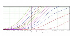
I tried adding the logarithmic ticks on the Dowell chart and it looks good except i can not get 1.1.
I have been calculating the position of the tick marks using the width from 1 to 2 and then taking the log of each tick mark and multiplying it times the width.
log 2 = .301 x width = 1.2 position
log 3 = .477 x width = 1.3 position
log 4 = .602 x width = 1.4 position
log 5 = .699 x width = 1.5 position
But the log of 1 is zero. I tried log of 1.5 and it clearly is not in the right place. In fact no position actually works out were the distance from 1 to 1.1 is a little bigger than the distance from 1.1 to 1.2 like logs should be.
Here are the relative measurements.
1 to 1.2 = 406 units
1.2 to 1.3 = 231 units
1.3 to 1.4 = 166 units
406 units - 231 units = 175 units, i am short. The distance from 1.1 to 1.2 has to be more than >231 units, and from 1 to 1.1 the distance has to be more than >>231 units.
Does anyone see the solution?
Attachments
- Status
- This old topic is closed. If you want to reopen this topic, contact a moderator using the "Report Post" button.
- Home
- Amplifiers
- Power Supplies
- Ferrite core for Boost PFC inductor.