Thanks DonVKAll the tubes were seperately driven with a constant velocity source in the graph below.
The "red" curve is a simple addition of all 8 separate tube's simulated outputs. The tubes still have relatively high Q and you can see that in the peaks.
The "green" curve is from driving all 8 tubes simultaneously (8 sources). The difference between the red and green is the effect of interaction between the physical tube openings. Keep in mind this is still 8 sources, not 1 shared source.
The "black" curve is when damping is applied to the tubes (all driven). I used D=5% Ft=1Khz which low. I'm not sure how much polyfill / fibreglass / cotton balls that is but it would be easy to put loose fill in a tube and measure the nearfield effect. Damping is also commonly used in TLs to smooth out these resonances.
In order to reproduce this from a single driver, the acoustic impedance of each tube needs to be similar because we will have 8 parallel loads on one driver. The impedance of a tube is a function of length and area ~f(L,A) . That part is next.
.
for sharing the work, I appreciate it even more by thinking about how many hours of study it will take to use the simulation program effectively. I have installed akabak and am looking for basic level documentation. To date, I have managed to improve my MDD projects with empirical tests, but it is becoming increasingly challenging to make new prototypes. I arrived at over 30 meters of waveguides for a pair of speakers, the MDD3FE25d prototype with 2 meters of maximum length sounds better than the previous ones, but I don't know if I have already exceeded the optimal length or it is worth going from floor to ceiling as in certain arrays. A mathematical model would be very useful to me.
The thing I appreciate most in these results is that the simulation shows that a series of guides with resonances can be used to obtain a linear response. The resonances distributed homogeneously in the frequency domain, overlap more and more by introducing a damping element and compensate each other. With the REW program I did something like this with the function that calculates the average of multiple responses measured at the end of the individual waveguides, see neutral cabinet. In this simulation you use odd resonances in relation to L / 4. In my prototypes at low frequencies the resonances in relation to L / 2 typical of the waveguides open on both sides are more evident. The result does not change as they can always be distributed homogeneously on one or more octaves and introduce adequate damping.
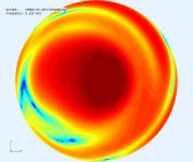
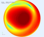
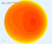
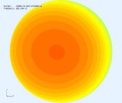
On the simulation made for the K-Tube and also with the STL file of Pelanj I did not understand the distribution of sound energy with increasing frequency, the average color of the maps goes from orange red (3KHz) to light blue (16KHz). My interpretation is that at high frequencies there is in total less total sound energy than at medium frequencies, is that correct?
Attachments
Can we make a compact horn using k-tube or MDD with 2" comp driver from 300Hz to 1,5kHz? Normally it is expo horn ca. 37cm long and 1000cm2.
Hi Jzagaja
the test closest to the conditions you wrote is that with the MDDHX135 prototype in which I mounted seven waveguides raised by one cm compared to a broad band of the Ciare now out of production. The driver is similar in size to what you used in your test with the 5FE120. I don't know if you only placed it with the edge open or mounted sealed. The total section of my guides is about 3 "instead of 2". The length reaches 500 mm.
I checked the measurement of the distortion inside the waveguides and it reaches 10% at the resonances. The high Q of the open guide triggers the vibrations in the internal air too easily. When I start working on the prototype MDDHX135 I will add damping material.
For omnidirectional emission, the DonVK simulation highlights 2 KHz lobes so at the moment I don't have a specific suggestion for your application. With a series of tests, an effective omnidirectional configuration should be reached, but work is still to be done.
Attachments
Can we make a compact horn using k-tube or MDD with 2" comp driver from 300Hz to 1,5kHz? Normally it is expo horn ca. 37cm long and 1000cm2.
Yes you could, but with caveats as always. The basic tube (one end closed would be (344)/(4*300)=0.28m avg length (probably 0.3m to the chamfer tip).
The problem is the distance between peaks when you only have 1 tube. The K-tube uses the slot to help spread out the resonance (still has ripple). You would need more damping to smooth out the ripple and it would cause HF attenuation (as @pelanj discovered). It might be more feasible to use, say 3 tubes, as a compromise. The more tubes the smoother it gets.
The other issue is getting a compression driver to run down at 300Hz. That's a very special (expensive
") ) driver.
) driver.DonVK, as always, very interesting post. I damped mine with a small cube of open cell foam and I perceived too much high end loss, so I halved the cubes and that is how it stayed. I am currently printing the second holder, the first one was good on first try, the second one looks like cursed.
I'm not surprised a single tube has significant ripple. It's always a tradeoff between smoothness and attenuation. It would be nice to have "bandpass" damping material.
Thanks for printing, testing and posting your results. I'm not at the stage where I can do 3D printing yet, but it's on my list.
Last edited:
Thanks DonVK
for sharing the work, I appreciate it even more by thinking about how many hours of study it will take to use the simulation program effectively. I have installed akabak and am looking for basic level documentation. To date, I have managed to improve my MDD projects with empirical tests, but it is becoming increasingly challenging to make new prototypes. I arrived at over 30 meters of waveguides for a pair of speakers, the MDD3FE25d prototype with 2 meters of maximum length sounds better than the previous ones, but I don't know if I have already exceeded the optimal length or it is worth going from floor to ceiling as in certain arrays. A mathematical model would be very useful to me.
You're welcome. I'm always interested in how a new idea works. The simulations are a good way to see whats going on.
Keep in mind that you need to create the design (I use Freecad), then create a mesh (I use Gmsh) then you can use the design in an ABEC (now Akabak) model for analysis.
The thing I appreciate most in these results is that the simulation shows that a series of guides with resonances can be used to obtain a linear response. The resonances distributed homogeneously in the frequency domain, overlap more and more by introducing a damping element and compensate each other. With the REW program I did something like this with the function that calculates the average of multiple responses measured at the end of the individual waveguides, see neutral cabinet. In this simulation you use odd resonances in relation to L / 4. In my prototypes at low frequencies the resonances in relation to L / 2 typical of the waveguides open on both sides are more evident. The result does not change as they can always be distributed homogeneously on one or more octaves and introduce adequate damping.
One thing I should mention is that in this case I just used REW to display multiple curves. All the data and processing was done in ABEC/VACS. I've also used REW, as you did, to avg the nearfield responses to get the overall response of an n-way speaker.
Also, keep in mind that what I show from simulations it's only the direct radiation from the tubes in 4Pi space. That's why its important to time gate any actual measurements for comparison. It appears that your measurement are not gated and include all the reflected energy from the room.
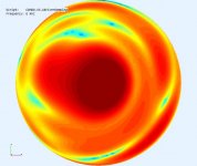
On the simulation made for the K-Tube and also with the STL file of Pelanj I did not understand the distribution of sound energy with increasing frequency, the average color of the maps goes from orange red (3KHz) to light blue (16KHz). My interpretation is that at high frequencies there is in total less total sound energy than at medium frequencies, is that correct?
Yes the lighter colors are lower pressure (assuming you are looking at the dome observation fields). They show the output level decreasing as the directivity increases and that does seem odd unless there is destructive interference occurring or the radiation impedance is decreasing. I'll post similar data for the 8 chamfered tubes I just posted.
Yes you could, but with caveats as always. The basic tube (one end closed would be (344)/(4*300)=0.28m avg length (probably 0.3m to the chamfer tip).
The problem is the distance between peaks when you only have 1 tube. The K-tube uses the slot to help spread out the resonance (still has ripple). You would need more damping to smooth out the ripple and it would cause HF attenuation (as @pelanj discovered). It might be more feasible to use, say 3 tubes, as a compromise. The more tubes the smoother it gets.
The other issue is getting a compression driver to run down at 300Hz. That's a very special (expensive
Good thing about MDD is that waveguide is equal to Sd - with horn it is 15x more. I'm thinking about car installation in very a tight space. Driver is not a problem but not larger than 2" throat. Linearity is also not a problem but I need 130dB peak.
Good thing about MDD is that waveguide is equal to Sd - with horn it is 15x more. I'm thinking about car installation in very a tight space. Driver is not a problem but not larger than 2" throat. Linearity is also not a problem but I need 130dB peak.
130db,...in a car,....
.
reducing ripple - single larger driver
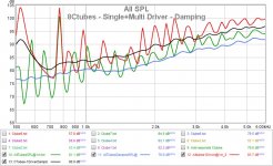
Following up, this is comparing the 8 separate Ctube drivers (1 per tube) to a single driver with a common chamber for the 8 tubes.
The 8 separate drivers have total drive area (8*Pi*1^2=25cm^2) while the single driver has area (1*Pi*3.75^2)=44.15 cm^2). So we should get ~20log(44.15/25)=4.9dB gain from the compression using a larger single driver.
The "green" curve is from the previous post. It's the 8 tube drivers simultaneously driving 8 tubes and will include the interaction from the outputs.
The "blue" curve is the "green" setup with low damping applied in the tubes.
The "red" curve is a larger single driver (ideal constant velocity) for 8 tubes and now includes interaction in the drive chamber due to different tube acoustic impedances. Notice that many of the peaks no longer line up with the table prediction because (IMO) there is uneven loading between the tubes. Still, it's not too bad above 700Hz, I was pleasantly surprised.
The "black" curve is the "red" setup with low damping added. Note the offset of approx 5dB (w.r.t blue) from the larger driver and compression effect. Also note there is a good correlation between "blue" and "black" above 700 Hz. To fix the region below 700Hz the tube areas would need to changed, or EQ added . Its also difficult to get effective damping material at lower freq which is consistent with the damping used in the model.
Up next, simulating with a 75mm cone driver model (electrical and acoustic).
.
Attachments
Last edited:
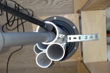
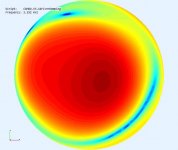
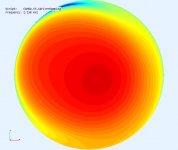
.. and the R60cm hemisphere dome observation fields. The shortest tube is on the X-axis facing right and we are looking from the top down into the tube openings.
.
.
Attachments
Following up, this is comparing the 8 separate Ctube drivers (1 per tube) to a single driver with a common chamber for the 8 tubes.
The 8 separate drivers have total drive area (8*Pi*1^2=25cm^2) while the single driver has area (1*Pi*3.75^2)=44.15 cm^2). So we should get ~20log(44.15/25)=4.9dB gain from the compression using a larger single driver.
The "green" curve is from the previous post. It's the 8 tube drivers simultaneously driving 8 tubes and will include the interaction from the outputs.
The "blue" curve is the "green" setup with low damping applied in the tubes.
The "red" curve is a larger single driver (ideal constant velocity) for 8 tubes and now includes interaction in the drive chamber due to different tube acoustic impedances. Notice that many of the peaks no longer line up with the table prediction because (IMO) there is uneven loading between the tubes. Still, it's not too bad above 700Hz, I was pleasantly surprised.
The "black" curve is the "red" setup with low damping added. Note the offset of approx 5dB (w.r.t blue) from the larger driver and compression effect. Also note there is a good correlation between "blue" and "black" above 700 Hz. To fix the region below 700Hz the tube areas would need to changed, or EQ added . Its also difficult to get effective damping material at lower freq which is consistent with the damping used in the model.
Up next, simulating with a 75mm cone driver model (electrical and acoustic).
.
Hi DonVK
I like this simulation, it is the one closest to my working hypotheses. The common compression chamber activates the exchange of sound energy between the eight waveguides, improving the effectiveness of the omnidirectional emission into the environment. The resonances should be in relation to L / 2 typical of the waveguides open on both sides. In my measurements these resonances are particularly evident in the trend of the driver's electrical impedance without damping material. To this resonance is added that to L / 4 relative to the maximum length of the waveguides with a reduction distributed in the spectrum caused by the interaction with the other waveguides of different length.
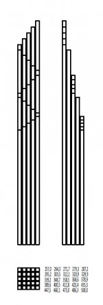
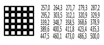
If I had to build a prototype with eight waveguides with a maximum length of 85.8 mm I would use the following lengths: 46.8 - 51.0 - 55.6 - 60.7 - 66.2 - 72.1 - 78.7 - 85.8 mm. The values can be scaled. In the simulation there is the further complication of the inclined profile.
A single waveguide, on a single driver, has a frequency response strongly conditioned by the typical resonance in relation to its length. With the lengths distributed evenly over an octave, for all frequencies there is a preferential path to transfer sound energy from the compression chamber to the environment. The delayed multiple emission, potentially omnidirectional that exploits the acoustic diffraction completes the characteristics of the sound emission of the MDD technology.
From the graphs relating to the hemisphere at the various frequencies, it is seen that the energy emitted horizontally attenuates with the frequency but at the same time increases the sound energy sent upwards. In a closed room with a normally reflective ceiling, this energy arrives delayed at the listening point. There are loudspeakers that require the use of an additional tweeter to recreate this effect.
Attachments
130 dB
Hi Jzagaja
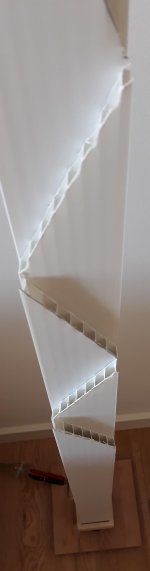
130 dB is 40 dB more than what was tested with my prototypes, they are sound pressure higher than two orders of magnitude and there may be unexpected behavior. Working at 130 dB, turbulence phenomena with high distortion could be triggered. However, I designed a front load of 500 mm high with a 5 x 5 matrix made with square aluminum guides of 10 x 10 mm. With the 3D printer or a CNC cutter a flange should be built to adapt the driver to the square section of the frontal acoustic load. The flange should have a compression chamber of about 10 mm between the driver and the beginning of the waveguides to allow the exchange of sound energy between the guides, see DonVK sim.
In linear mode the individual guides show peaks in the response to frequencies in relation to the lengths of the guides themselves. By introducing dissipative elements the peaks reduce, widen and overlap compensating each other. Alternatively, the number of guides can be increased so that the number of peaks increases and they overlap even without dissipative elements, see project 54m42 made of 10 mm alveolar polypropylene. To maximize the sound pressure in the drawing, I hypothesized 25 square waveguides without damping elements.
To get the maximum sound pressure, I think aluminum is more suitable. To get an idea of the feasibility, a 10 mm alveolar polypropylene prototype can be created. The zigzag pattern allows to use this material, five 50 mm strips with the high oblique side would suffice. In the event that 25 guides are not sufficient, 5 mm alveolar polypropylene could be used to build a 10 x 10 matrix with 100 wave guides with lengths in logarithmic series.
Based on the DonVK sim, part of the high frequency energy would be sent upwards and outdoors would not reach the listener. Depending on the intended use, the high side of the frontal acoustic load can be oriented towards the listening point, renouncing the MDD effect or introducing reflective panels that would however increase the size.
Good thing about MDD is that waveguide is equal to Sd - with horn it is 15x more. I'm thinking about car installation in very a tight space. Driver is not a problem but not larger than 2" throat. Linearity is also not a problem but I need 130dB peak.
Hi Jzagaja
130 dB is 40 dB more than what was tested with my prototypes, they are sound pressure higher than two orders of magnitude and there may be unexpected behavior. Working at 130 dB, turbulence phenomena with high distortion could be triggered. However, I designed a front load of 500 mm high with a 5 x 5 matrix made with square aluminum guides of 10 x 10 mm. With the 3D printer or a CNC cutter a flange should be built to adapt the driver to the square section of the frontal acoustic load. The flange should have a compression chamber of about 10 mm between the driver and the beginning of the waveguides to allow the exchange of sound energy between the guides, see DonVK sim.
In linear mode the individual guides show peaks in the response to frequencies in relation to the lengths of the guides themselves. By introducing dissipative elements the peaks reduce, widen and overlap compensating each other. Alternatively, the number of guides can be increased so that the number of peaks increases and they overlap even without dissipative elements, see project 54m42 made of 10 mm alveolar polypropylene. To maximize the sound pressure in the drawing, I hypothesized 25 square waveguides without damping elements.
To get the maximum sound pressure, I think aluminum is more suitable. To get an idea of the feasibility, a 10 mm alveolar polypropylene prototype can be created. The zigzag pattern allows to use this material, five 50 mm strips with the high oblique side would suffice. In the event that 25 guides are not sufficient, 5 mm alveolar polypropylene could be used to build a 10 x 10 matrix with 100 wave guides with lengths in logarithmic series.
Based on the DonVK sim, part of the high frequency energy would be sent upwards and outdoors would not reach the listener. Depending on the intended use, the high side of the frontal acoustic load can be oriented towards the listening point, renouncing the MDD effect or introducing reflective panels that would however increase the size.
Attachments
Hi DonVK
The resonances should be in relation to L / 2 typical of the waveguides open on both sides.
The simulation uses a L/4 because the tube is closed at one end (closed driver chamber). The simulation results and the predicted table align based on L/4. This places the peaks at "odd" numbered length multiples. So the tube spectrum was spread over 3*f instead of an octave (2*f).
In the simulation there is the further complication of the inclined profile.
The rising response with freq is from the model using an ideal membrane with constant velocity. A real world driver operates in regions of constant velocity and regions of constant acceleration (ie. force) plus a bunch of other complications. That's next up.
From the graphs relating to the hemisphere at the various frequencies, it is seen that the energy emitted horizontally attenuates with the frequency but at the same time increases the sound energy sent upwards. In a closed room with a normally reflective ceiling, this energy arrives delayed at the listening point. There are loudspeakers that require the use of an additional tweeter to recreate this effect.
The sound should becomes more directional as freq increases unless some design effort is taken to create more constant directivity. The relative amount of reflection is a personal preference. I would tilt this type of speaker at 45deg to partially aim direct sound it at the listener like a K-tube.
.
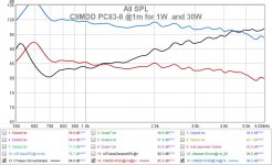
PC83-8 driver model with C8MDD
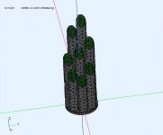
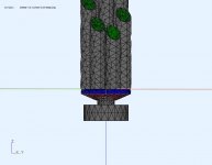
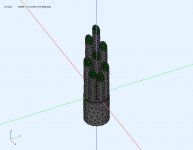
The single ideal driver membrane was replaced with a model of a Dayton PC83-8 full range driver. I have a pair of these and the model requires actual driver physical measurements (BEM) and electrical T/S parameters (LEM).
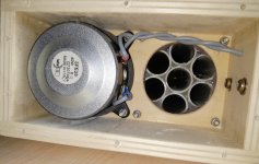
The driver model includes a small closed damped rear chamber (0.2L) and 5mm deep front chamber like before. Pics are below, with the rear chamber on, and then removed to show the cone, VC and magnet.
The "black" curve was presented earlier (post 128) as the ideal single driver membrane with constant velocity.
The "red" curve is the PC83-8 driving the tubes. The datasheet specifies 85dB/1m @2.83vrms (open air) and that's actually close to what we see. The driver and chamber model changed the system resonance as we would expect. There is a moderate bump +6db@600Hz that could be EQ'd or notch filtered out. There is a slight HF droop that IMO is from a combination of increasing VC reactance (need a better shorting cap model) and limited force (limited acceleration). The residual tube ripple is similar for red and black curves.
The "blue" curve is at Pmax=30W (14.2Vrms) for @jzagaja.
.
The single ideal driver membrane was replaced with a model of a Dayton PC83-8 full range driver. I have a pair of these and the model requires actual driver physical measurements (BEM) and electrical T/S parameters (LEM).
The driver model includes a small closed damped rear chamber (0.2L) and 5mm deep front chamber like before. Pics are below, with the rear chamber on, and then removed to show the cone, VC and magnet.
The "black" curve was presented earlier (post 128) as the ideal single driver membrane with constant velocity.
The "red" curve is the PC83-8 driving the tubes. The datasheet specifies 85dB/1m @2.83vrms (open air) and that's actually close to what we see. The driver and chamber model changed the system resonance as we would expect. There is a moderate bump +6db@600Hz that could be EQ'd or notch filtered out. There is a slight HF droop that IMO is from a combination of increasing VC reactance (need a better shorting cap model) and limited force (limited acceleration). The residual tube ripple is similar for red and black curves.
The "blue" curve is at Pmax=30W (14.2Vrms) for @jzagaja.
.
Attachments
Last edited:
The single ideal driver membrane was replaced with a model of a Dayton PC83-8 full range driver. I have a pair of these and the model requires actual driver physical measurements (BEM) and electrical T/S parameters (LEM).
The driver model includes a small closed damped rear chamber (0.2L) and 5mm deep front chamber like before. Pics are below, with the rear chamber on, and then removed to show the cone, VC and magnet.
The "black" curve was presented earlier (post 128) as the ideal single driver membrane with constant velocity.
The "red" curve is the PC83-8 driving the tubes. The datasheet specifies 85dB/1m @2.83vrms (open air) and that's actually close to what we see. The driver and chamber model changed the system resonance as we would expect. There is a moderate bump +6db@600Hz that could be EQ'd or notch filtered out. There is a slight HF droop that IMO is from a combination of increasing VC reactance (need a better shorting cap model) and limited force (limited acceleration). The residual tube ripple is similar for red and black curves.
The "blue" curve is at Pmax=30W (14.2Vrms) for @jzagaja.
.
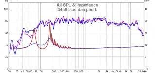
The compression chamber is closed but a part of the internal edges of the waveguides is free and allows the exchange of energy with the neighboring guides. In particular, the external guides have about half closed edge and half open edge, a significant complication. My measurements with the microphone are less reliable than the impedance measurement of the loudspeaker. In the graph of project 34c9 the response in the environment does not allow me to detect resonances, the impedance graph highlights a series of peaks between 171 and 309 Hz relative to L / 2 of each individual guide with a length between 552 and 1000 mm. In the next few days I will try to detect the same resonances by redoing the measurements with the microphone inside the individual guides in the MDD3FE25d project.
One of the reasons why the MDD3FE25d project sounds better than the previous ones can be that the frontal acoustic load guides have lengths between 300 and 1600 mm and optimize the ratio of direct reflected sound for my room 4 x 4 x 3 meters. In a measure made with the ARTA program I have the RASTI index at 0.76, the minimum for the recording rooms but in a room that is not acoustically treated.
With MDD technology, the 600 Hz bump can be attenuated without using filters. Once the simulation model has been refined, the lengths of some guides can be modified so that they compensate for the non-linearity of the response. The diffraction emission can also be modified by introducing lateral holes on the external waveguides, a further complication for the simulation.
Attachments
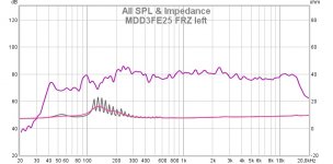
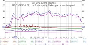
MDD3FE25d resonances
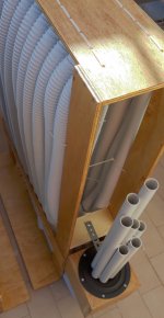
Loudspeakers with MDD technology are easy to build, they are inexpensive but complex to describe with a mathematical model. The complexity of the MDD3FE25d project derives from the presence of 14 wave guides with different length and with resonances generated by the double configuration: wave guides with one side closed and one side open, wave guides with two sides open. The six external waveguides of the frontal acoustic load and of the rear acoustic load have part of the lower edge free and part closed (outside). The central waveguide has the entire free bottom edge.
Further complications are the interaction at the top exit of the shorter guides due to the close presence of the longer guides, also the diffraction emission is affected by upward directionality phenomena at high frequencies.
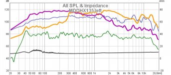
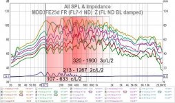
The complexity of the mathematical model of the project is visible in the trend of the electrical impedance measured without damping material (red line). The origin of the peaks derives from the frontal acoustic load and the rear acoustic load. The peaks generated by the rear acoustic load (green line) can be measured by inserting damping material in the front load. Vice versa, the peaks generated by the frontal acoustic load (blue line) can be measured by inserting damping material in the rear load. The purple line is in normal listening conditions with both damped acoustic loads.
In the absence of a mathematical model of the prototype, excellent configurations can be obtained empirically with good FR measurements in the environment. In the MDD3FE25d prototype, the electrical impedance (purple line) has only slight ripples instead of the two evident maxima of the TL systems. The blue line is the FR in the environment of the left channel positioned in the corner of the room. The purple line is the FR in the environment of the right channel positioned near the wall about one meter from the other corner of the room 4 x 4 x 3 meters. The differences between the channels are caused by the interaction of the loudspeakers with the room.
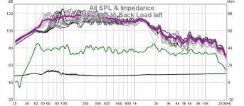
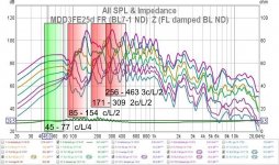
To connect the resonances measured in the electrical impedance of the MDD3FE25d project to the resonances measured acoustically, I detected the FR at the end of each waveguide with the microphone inside about one cm. This is not a professional measure, it is sufficient to highlight the behavior of the individual waveguides of the front and rear acoustic loads. All measurements inside the waveguides were made without damping material.
The green area of the measurements on the rear acoustic load 21BL7d shows the only detectable effects of the resonances with f = c / L / 4 where c = 341 m / sec. The waveguides have lengths between 2 and 1.1 meters which correspond to the frequencies between 45 and 77 Hz. In the impedance graph there is a relative peak of about 9.8 Ohm at 48 Hz. The peak is reduced compared to standard TL systems as it is the result of waveguide interactions with different length. The second relative peak, typical of TL systems, is only mentioned, masked by the peaks related to the resonances of the waveguides with the sides open f = n * c / L / 2. In the graph FR there is a change of slope for the same frequency about 45 Hz.
The red areas of the measurements on the rear acoustic load 21BL7d show the effects of resonances with f = n * c / L / 2 where n = 1, 2, 3 and c = 341 m / sec. The waveguides have lengths between 2 and 1.1 meters which correspond to the frequencies between 85 and 154, 171 and 309, 256 and 463 Hz. In the impedance graph there are 7 relative peaks in each interval. In the graph FR there are 7 relative peaks for each interval, they are partially superimposed starting from n = 3.
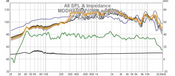
The red areas of the measurements on the frontal acoustic load 23FL7d show the effects of resonances with f = n * c / L / 2 where n = 1, 2, 3 and c = 341 m / sec. The waveguides have lengths between 1.6 and 0.27 meters which correspond to the frequencies between 107 and 633, 213 and 1267, 320 and 1900 Hz. In the impedance graph there are 7 relative peaks in each interval, easily distinguishable up to 200 Hz. In the graph FR there are 7 relative peaks for each interval, they are partially superimposed already with n = 1.
Other links:
https://www.claudiogandolfi.it/
https://www.claudiogandolfi.it/mdd3fe25.html#d (REW file with damped and no damped measures)
https://www.claudiogandolfi.it/mddfl.html#23fl7d
https://www.claudiogandolfi.it/mddbl.html#21bl7d
Loudspeakers with MDD technology are easy to build, they are inexpensive but complex to describe with a mathematical model. The complexity of the MDD3FE25d project derives from the presence of 14 wave guides with different length and with resonances generated by the double configuration: wave guides with one side closed and one side open, wave guides with two sides open. The six external waveguides of the frontal acoustic load and of the rear acoustic load have part of the lower edge free and part closed (outside). The central waveguide has the entire free bottom edge.
Further complications are the interaction at the top exit of the shorter guides due to the close presence of the longer guides, also the diffraction emission is affected by upward directionality phenomena at high frequencies.
The complexity of the mathematical model of the project is visible in the trend of the electrical impedance measured without damping material (red line). The origin of the peaks derives from the frontal acoustic load and the rear acoustic load. The peaks generated by the rear acoustic load (green line) can be measured by inserting damping material in the front load. Vice versa, the peaks generated by the frontal acoustic load (blue line) can be measured by inserting damping material in the rear load. The purple line is in normal listening conditions with both damped acoustic loads.
In the absence of a mathematical model of the prototype, excellent configurations can be obtained empirically with good FR measurements in the environment. In the MDD3FE25d prototype, the electrical impedance (purple line) has only slight ripples instead of the two evident maxima of the TL systems. The blue line is the FR in the environment of the left channel positioned in the corner of the room. The purple line is the FR in the environment of the right channel positioned near the wall about one meter from the other corner of the room 4 x 4 x 3 meters. The differences between the channels are caused by the interaction of the loudspeakers with the room.
To connect the resonances measured in the electrical impedance of the MDD3FE25d project to the resonances measured acoustically, I detected the FR at the end of each waveguide with the microphone inside about one cm. This is not a professional measure, it is sufficient to highlight the behavior of the individual waveguides of the front and rear acoustic loads. All measurements inside the waveguides were made without damping material.
The green area of the measurements on the rear acoustic load 21BL7d shows the only detectable effects of the resonances with f = c / L / 4 where c = 341 m / sec. The waveguides have lengths between 2 and 1.1 meters which correspond to the frequencies between 45 and 77 Hz. In the impedance graph there is a relative peak of about 9.8 Ohm at 48 Hz. The peak is reduced compared to standard TL systems as it is the result of waveguide interactions with different length. The second relative peak, typical of TL systems, is only mentioned, masked by the peaks related to the resonances of the waveguides with the sides open f = n * c / L / 2. In the graph FR there is a change of slope for the same frequency about 45 Hz.
The red areas of the measurements on the rear acoustic load 21BL7d show the effects of resonances with f = n * c / L / 2 where n = 1, 2, 3 and c = 341 m / sec. The waveguides have lengths between 2 and 1.1 meters which correspond to the frequencies between 85 and 154, 171 and 309, 256 and 463 Hz. In the impedance graph there are 7 relative peaks in each interval. In the graph FR there are 7 relative peaks for each interval, they are partially superimposed starting from n = 3.
The red areas of the measurements on the frontal acoustic load 23FL7d show the effects of resonances with f = n * c / L / 2 where n = 1, 2, 3 and c = 341 m / sec. The waveguides have lengths between 1.6 and 0.27 meters which correspond to the frequencies between 107 and 633, 213 and 1267, 320 and 1900 Hz. In the impedance graph there are 7 relative peaks in each interval, easily distinguishable up to 200 Hz. In the graph FR there are 7 relative peaks for each interval, they are partially superimposed already with n = 1.
Other links:
https://www.claudiogandolfi.it/
https://www.claudiogandolfi.it/mdd3fe25.html#d (REW file with damped and no damped measures)
https://www.claudiogandolfi.it/mddfl.html#23fl7d
https://www.claudiogandolfi.it/mddbl.html#21bl7d
Attachments
@claudiogan, thanks for posting the measurements, an explanation and the links. This configuration has tubes on both sides of the driver and is a different configuration than I simulated previously (ie. tubes one one side). However it's easy enough to simulate tubes on both sides when I get some time. I'm curious about the interaction between 2 tubes of different length on opposite sides of the same driver membrane.
Haas effect
Reading an article on the Haas effect, I identified the cause of the improvement in listening quality in the MDD3FE25 project linked to the increase in the length of the frontal acoustic load.
With MDD technology, the sound fronts emitted with delays between 1 and 6 msec prevent the perception of the Haas effect that can generate sound reflections on the walls.
Between the beginning and the end of the envelope of a note, the intervals without sound energy are eliminated, the decoding of sounds is simplified.
More information on the page
acustica MDD projects
In the FAQ page I have added some answers to clarifications on MDD technology requested by email
https://www.claudiogandolfi.it/faq.html
After a couple of months I managed to complete version d of the MDD3FE25 project. As expected, the increase in length of the rear acoustic load to 2 meters has improved the response to low frequencies. The time available allowed me to try various configurations for the front acoustic load, the best result is that with a front loading 23FL7d (1600 mm with resonances over 3 octaves), the maximum length is close to the maximum length of the rear loading 21BL7d ( 2000 mm with resonances on one octave). The perception of high-pitched sounds has also improved, from the measurements I do not detect the difference that is perceived when listening. The difference in distortion does not justify it, on the contrary it is just higher. Guides up to 2 meters long create more vibration and are more difficult to glue deafly. Pending confirmation or denial, I attribute the credit to the further optimized MDD effect.
Reading an article on the Haas effect, I identified the cause of the improvement in listening quality in the MDD3FE25 project linked to the increase in the length of the frontal acoustic load.
With MDD technology, the sound fronts emitted with delays between 1 and 6 msec prevent the perception of the Haas effect that can generate sound reflections on the walls.
Between the beginning and the end of the envelope of a note, the intervals without sound energy are eliminated, the decoding of sounds is simplified.
More information on the page
acustica MDD projects
In the FAQ page I have added some answers to clarifications on MDD technology requested by email
https://www.claudiogandolfi.it/faq.html
@claudiogan
Congratulations on the study you are doing.
I searched youtube but couldn't find anything about how your device sounds.
it would be interesting to have a sound test to understand, beyond the numbers and graphics, how it behaves when listening, perhaps with an uncompressed file. I continue to follow the discussion with interest
Thank you
- Home
- Loudspeakers
- Planars & Exotics
- MDD Multi Delays Diffraction (Multi TL, omnidirectional, single drive, ...)