I'm sure that when I open your spreadsheets, the angels sing and the lambs lie down with the lion. But most of us know how to use tabs (even old fogies like me), and having an overview on the first tab can be useful.
Having something that actually works on the first page ain't exactly rocket science. Since casting aspersions on people's professional qualifications seems to be stylish around here, let me add that any professional should know that!
Perhaps its a case of knowing better, and sensibly using software that respects the users freedom. https://www.youtube.com/watch?v=uJi2rkHiNqgInteresting that someone claiming to be an engineer doesn't know how to work tabs in Excel.
Cryptic stuff that only the original writer can understand is great for the original writer. For everybody else, not so much. IMO, too many comments is more useful than too few. But hey, it isn't locked or anything. Every tab has a delete selection. So does the whole thing if you like. Re-format it, re-purpose it, re-move it, or whatever makes it useful to you.
More importantly, my real goal with this thing was to let people fool with bypass cap math and reach their own conclusions. Just stating that it's usually a fools errand for audio stuff hasn't accomplished much. What I should probably do is add a tab with measured results for a variety of caps at various frequencies, since those numbers seem to be hard to come by.
More importantly, my real goal with this thing was to let people fool with bypass cap math and reach their own conclusions. Just stating that it's usually a fools errand for audio stuff hasn't accomplished much. What I should probably do is add a tab with measured results for a variety of caps at various frequencies, since those numbers seem to be hard to come by.
No, you have to use the model which fits the situation. If you are adding something in parallel, then use the parallel model. If adding something in series, use the series model. Changing models as you design (or analyse) a circuit is part of engineering. As I said, RF people do this all the time (especially when designing matching networks). Audio folk don't, partly because losses are less significant and partly because (on average) audio folk seem to know less about electronics.Conrad Hoffman said:IMO, the parallel model is best for high loss/low Q situations, but when considering components for audio, where we go from quite low frequencies, to high, it could be confusing to people to change models somewhere in the range. In theory, either model predicts what happens just fine, though the "gut feel" for the model values will be a bit odd when the "wrong" model is used. Thus comes about the oddities when using the series model at high frequencies with highly imperfect components.
Yes, single frequency. As the frequency changes the model values change. How they change depends on what exactly is happening. If the series model is a good approximation to reality (e.g. an electrolytic at audio frequencies) then the series model values will be fairly constant, but the parallel model values will change a lot. On the other hand, you could find that some components are best modelled by a parallel model (e.g. electrolytic at subsonic frequencies where leakage dominates?) and then it would be the series values which change a lot.One can't emphasize enough that both these models are valid for a single frequency only. At that single frequency, whatever capacitive (-) and inductive (+) reactance add, leaving only a single value, be it one or the other, and are not considered separately. The loss term covers pretty much everything else, even including dielectric absorption, leaving only some non-linearities unaccounted for. With a true bridge, those show up as a non-zero residual when the bridge is balanced.
I suspect not, unless series inductance is a factor. When inductance comes into play, 'bypassing' a big cap with a small one can give an apparent net capacitance which is smaller than the big cap on its own. This is because you are approaching parallel resonance. A cap meter won't know this so just thinks the capacitance has got smaller.In your example, take the losses a bit higher. I think you'll find the total Cs does in fact decrease.
With everything at a single frequency, inductive reactance has combined with capacitive reactance, hopefully disappeared, and doesn't come into play. If you artificially increase the losses of a cap by adding a series resistor, the measurement (and math) can be done far away from resonance, and the Cs decrease still happens. It's just a quirk of the math behind the models, which is what I originally found so interesting.
If the single frequency is sufficiently high then inductive reactance has combined in series with capacitive reactance to provide net inductive reactance. Far from disappearing - you now have a DC-blocking inductor! Even below this point the inductive reactance has apparently increased the series value of the capacitor, which may reduce the parallel value. This stuff is counter-intuitive, so it is not surprising that people get confused. Not a quirk of the maths, but just because reality is more complicated than naive models.Conrad Hoffman said:With everything at a single frequency, inductive reactance has combined with capacitive reactance, hopefully disappeared, and doesn't come into play.
I'm by no means confused, though I certainly don't have your DC-daylight knowledge of this stuff. IMO, unless one starts speaking about specific parts and frequencies (guilty as charged) it's easy to be discussing different aspects of the same thing. BTW, that DC-blocking inductor, which is common with big electrolytics at audio frequencies, still tends to be a very low value, a few uH, and very low Q, so it's more like a low value resistor than anything else. The question I've always wondered about is whether there's any real difference or advantage in terms of coupling, filtering or bypassing, between that, and a capacitor that actually maintains low losses and remains a capacitor at those higher frequencies. My guess is probably not, otherwise nothing would work as well as it does beyond some tens of kHz.
BTW, DC-daylight is a compliment, as I know you could shift over to distributed parameter models without a hitch. Fortunately, for this mathphobe, lumped models are usually all one needs for audio. As for the models being naive, they predict low frequency physical circuit performance to an astoundingly high degree. RF, maybe not so good ;-)
Yes, lumped models are fine for audio. By 'naive' I simply meant those who think that a small tube marked 0.1uF is exactly that: an ideal 0.1uF capacitor with nothing else.
A 'DC-blocking inductor' is fine as a coupling capacitor. All that is required is that the impedance is significantly less than the load. For other purposes a check may be needed that the phase of the residual voltage being different from what is expected is not going to create problems.
A 'DC-blocking inductor' is fine as a coupling capacitor. All that is required is that the impedance is significantly less than the load. For other purposes a check may be needed that the phase of the residual voltage being different from what is expected is not going to create problems.
The net impedance is the same, but expressed in two different ways. There is a third way: impedance magnitude plus impedance phase.
That already assumes that you are using the parallel version of the component impedances, or assuming ideal lossless components.
For the benefit of baffled bystanders, this is what Conrad and I are discussing:
Any real impedance (e.g. a component) can be expressed as either the sum of a resistance and a reactance in series, or as a parallel combination. In the case of an electrolytic capacitor at lowish (i.e. audio) frequencies the best model is a capacitor in series with a small resistor. The resistor is ESR (say, 0.1R). The capacitor is the value marked on the can (say, 100uF).
As frequency increases the capacitive reactance decreases. ESR may increase a little, but we will assume for simplicity that it stays constant. There will come a frequency (15.9kHz) where capacitive reactance equals ESR. At this point the component no longer has the 90 degree phase of a pure capacitor but 45 degrees. It can be expressed in three ways:
0.1R + 100uF in series
0.2R in parallel with 50uF
0.1414R magnitude, 45 degrees phase
If you measure this with a capacitance meter what you will see depends on what frequency the meter uses and how it chooses to interpret the raw data.
Now add a perfect 1uF in parallel. This gives 0.2R with 51uF in parallel. Converting this back to series form gives 0.09798R + 100.02uF. The extra 1uF has almost disappeared! The main effect of the extra 1uF component is a small reduction in ESR. Given the real world with measurement error and some series inductance too it is easy to see why it might be thought that the total capacitance reduces. Note that all this applies at a single frequency only; you have to repeat the calculation for each frequency.
I just found this interesting thread.
When I do the calculations for these example values, I get the same result with a slightly different value for the resistive part of the final result, no doubt due to slight rounding error in the calculations.
Taking Conrad's suggestion, I calculated the result for a 100 uF capacitor with a slightly higher ESR of .11R
This component can be expressed as:
0.11R + 100uF in series
.2009R in parallel with 45.249uF
Adding a perfect 1uF in parallel gives 0.2009R with 46.249uF in parallel.
Converting this back to series form gives 0.1078R + 99.816uF.
The capacitance of the series model has decreased.
If we start with a 100uF cap having an ESR of .15, then parallel that with a perfect 10uF, the final series equivalent is 0.1217R + 93.019uF. The equivalent capacitance is not increased by 10uF, but reduced by about 7uF.
This all has nothing to do with any parasitic inductance.
In the next post, I'll give a physical example.
I'm going to show the effect with real capacitors. To do so I will use an impedance analyzer to measure and display various capacitor parameters.
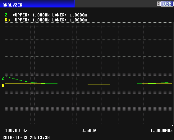
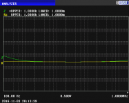
The impedance analyzer is set up to perform a sweep of frequency from 100Hz to 1MHz. The horizontal scale is logarithmic per convention. For the first sweep the vertical scale goes from .001 ohm at the bottom to 1000 ohms at the top. Two parameters are shown, impedance (Z, in green) and series equivalent resistance (ESR, in yellow). This sweep shows those parameters for a 5uF MKP capacitor. This is the capacitor that will be connected in parallel later. Here's the sweep:

We see at the left that the impedance (green) is decreasing with increasing frequency, as we would expect to happen with a capacitor. We see a sharp self resonance at about 300 kHz. The ESR starts out at 14 milliohms and decreases to about 9 milliohms by 10 kHz. This is a very good capacitor.
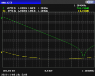
Now, the main capacitor is one I dug out of the stash box. It's nominal capacitance is 2000uF. It is not a good capacitor. Here is a sweep of its Z and ESR on the same scale. The impedance curve and ESR curve are practically coincident; the ESR is about .2 ohms, without much variation over the entire frequency range. There is a broad self resonance with the actual minimum at about 20 kHz:
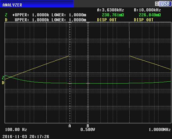
We can also perform a sweep showing Z and the dissipation factor D (yellow), rather than ESR. I've added two markers, marker A at 3.6 kHz and marker B at 10 kHz. The values of the parameters at the marker frequencies are shown at upper right. The impedance analyzer doesn't show D when it goes above 10, hence the disappearance of the yellow curve between 3.6 kHz and 100 kHz:
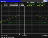
Now a sweep showing the capacitance of the inferior 2000uF capacitor vs. frequency. The vertical scale has been changed to be linear from zero at the bottom to 5000uF at the top, and the A marker has been moved to about 5 kHz:
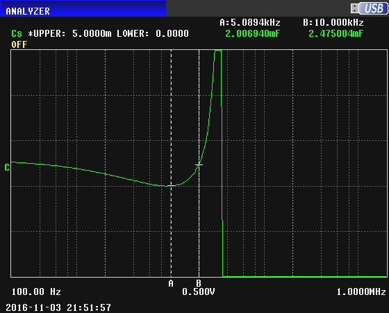
The capacitance at 100 Hz can be seen to be about 2500uF, and at 5 kHz it's 2007uF. The variation of the capacitance as frequency increases is typical for electrolytic capacitors with etched foil. The capacitance decreases as the frequency approaches the self resonance frequency (SRF), reaching a minimum at about 5 kHz, then increasing to a very large value at the SRF at about 20 kHz. Above the SRF, the apparent capacitance becomes negative (an inductive impedance).
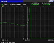
Now a sweep with the very good (low ESR) 5uF MKP capacitor in parallel with the inferior 2000uF capacitor. This sweep will be superimposed over the previous sweep. The capacitance curve for the parallel combination detaches at about 800 Hz from the curve of the previous sweep and takes on lower capacitance values from that frequency on. The capacitance at 5 kHz is 1328uF, a decrease of 679uF due to paralleling the 5uF MKP capacitor. Ordinarily, we would think that paralleling a 5 uF capacitor would increase the measured value of the 2000uF capacitor by 5 uF, but because the 2000uF capacitor has a high ESR this counterintuitive (to some of us) effect takes place. This is happening at frequencies well below those where parasitic inductance is having any effect.
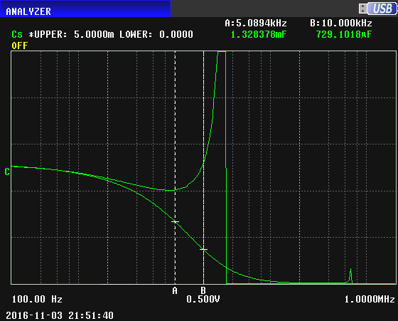
Notice that the original SRF at 20 kHz is gone. There's a new SRF just visible as a tiny blip at 352 kHz.
The effect Conrad describes is very apparent with these real capacitors.
The impedance analyzer is set up to perform a sweep of frequency from 100Hz to 1MHz. The horizontal scale is logarithmic per convention. For the first sweep the vertical scale goes from .001 ohm at the bottom to 1000 ohms at the top. Two parameters are shown, impedance (Z, in green) and series equivalent resistance (ESR, in yellow). This sweep shows those parameters for a 5uF MKP capacitor. This is the capacitor that will be connected in parallel later. Here's the sweep:
We see at the left that the impedance (green) is decreasing with increasing frequency, as we would expect to happen with a capacitor. We see a sharp self resonance at about 300 kHz. The ESR starts out at 14 milliohms and decreases to about 9 milliohms by 10 kHz. This is a very good capacitor.
Now, the main capacitor is one I dug out of the stash box. It's nominal capacitance is 2000uF. It is not a good capacitor. Here is a sweep of its Z and ESR on the same scale. The impedance curve and ESR curve are practically coincident; the ESR is about .2 ohms, without much variation over the entire frequency range. There is a broad self resonance with the actual minimum at about 20 kHz:
We can also perform a sweep showing Z and the dissipation factor D (yellow), rather than ESR. I've added two markers, marker A at 3.6 kHz and marker B at 10 kHz. The values of the parameters at the marker frequencies are shown at upper right. The impedance analyzer doesn't show D when it goes above 10, hence the disappearance of the yellow curve between 3.6 kHz and 100 kHz:
Now a sweep showing the capacitance of the inferior 2000uF capacitor vs. frequency. The vertical scale has been changed to be linear from zero at the bottom to 5000uF at the top, and the A marker has been moved to about 5 kHz:
The capacitance at 100 Hz can be seen to be about 2500uF, and at 5 kHz it's 2007uF. The variation of the capacitance as frequency increases is typical for electrolytic capacitors with etched foil. The capacitance decreases as the frequency approaches the self resonance frequency (SRF), reaching a minimum at about 5 kHz, then increasing to a very large value at the SRF at about 20 kHz. Above the SRF, the apparent capacitance becomes negative (an inductive impedance).
Now a sweep with the very good (low ESR) 5uF MKP capacitor in parallel with the inferior 2000uF capacitor. This sweep will be superimposed over the previous sweep. The capacitance curve for the parallel combination detaches at about 800 Hz from the curve of the previous sweep and takes on lower capacitance values from that frequency on. The capacitance at 5 kHz is 1328uF, a decrease of 679uF due to paralleling the 5uF MKP capacitor. Ordinarily, we would think that paralleling a 5 uF capacitor would increase the measured value of the 2000uF capacitor by 5 uF, but because the 2000uF capacitor has a high ESR this counterintuitive (to some of us) effect takes place. This is happening at frequencies well below those where parasitic inductance is having any effect.
Notice that the original SRF at 20 kHz is gone. There's a new SRF just visible as a tiny blip at 352 kHz.
The effect Conrad describes is very apparent with these real capacitors.
Attachments

Last edited:
I have sent Conrad an apology. He was right. I was wrong. Thanks for getting me to think about it again.
I'm glad I could contribute. It is an interesting, if not particularly useful, effect.
The mysteries of complex arithmetic; surprises galore.
- Status
- This old topic is closed. If you want to reopen this topic, contact a moderator using the "Report Post" button.
- Home
- Design & Build
- Parts
- Paralleling Caps / Bypassing Caps