Hello!
I do see here quite regularly threads about diffraction but, respectfully, I have the impression that sometimes there is not enough understanding about diffractions. I am no expert either but I spent quite some time researching and simulating on this matter and I think I can share some thoughts which may be helpful.
I don’t want this thread to be about the fundamental physical background of diffractions, I don’t want it to be about the design of a specific cabinet and I also don’t aim to make a new tool to calculate diffractions. There are already plenty.
Instead it should be about a general understanding of cause and effect regarding diffractions. I want to describe what can be expected from different measures to tame diffractions for proper sound reproduction.
I already have to apologize here because this will become quite a wall of text but at least there will be some pictures.
How to calculate diffractions
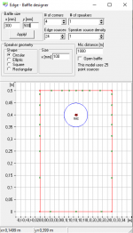
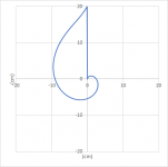
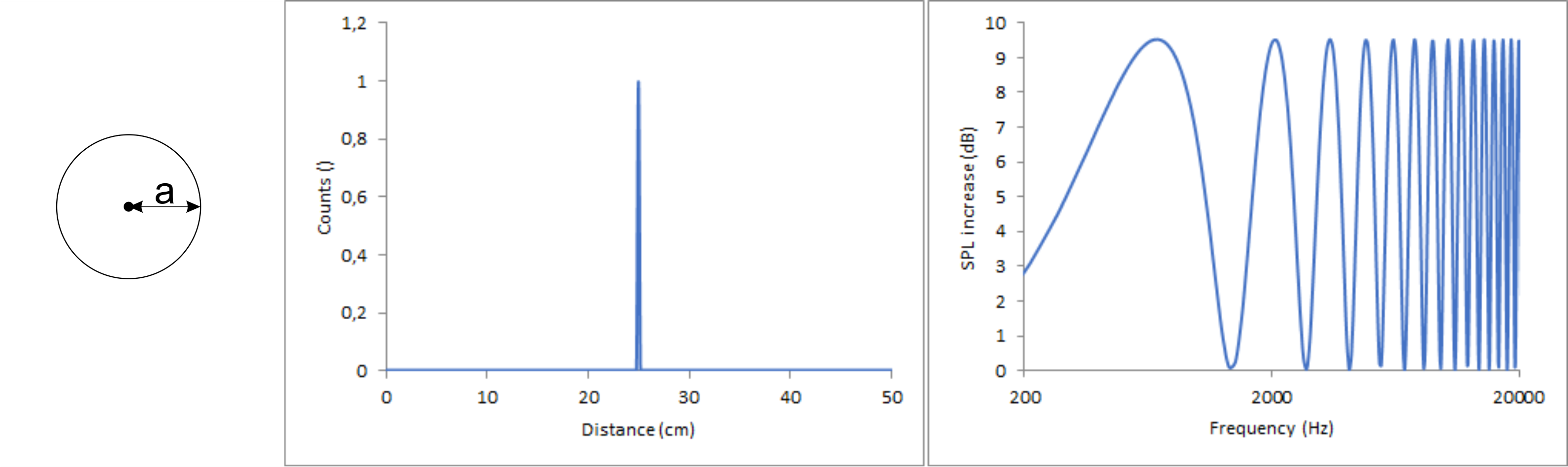
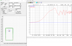
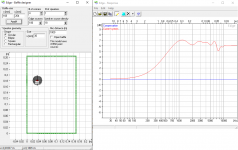
For a better understanding I think it’s best to start to explain how software like The Edge simulates diffractions. I am not affiliated with the software in any way so I can’t say anything about the details, only how this works in general. The input for such a simulation may look like this.

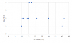
For each point at the edge of the baffle the software calculates the distance (Source –> Point at the baffle –> microphone) minus (Source –> microphone). For now, all my calculations will assume that the microphone is in infinite distance directly in front of the chassis. When doing exactly the same calculation in Excel, I get the following values as a function of the angle. I will call the result from this calculation “distance” from now on. 0° in this case is the perpendicular distance to the left edge and then every 15° there is another point at the edge in clockwise direction. It is quite easy to follow. The first 3 points are located at the left edge, each with slightly increasing distances, the next points are on top, which first decrease in distance until a distance of 10 cm is reached, representing the perpendicular distance to the top edge and so on. At an angle of about 270° three distances stand out representing the three points at the bottom edge.
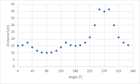
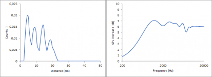
This plot can now be rearranged, because for diffractions it does not matter under which angle which distance is obtained. Only the distances themselves matter. For symmetry reasons some of the distances are the same and they can then be summarized. For example, 15°, 165°, 195° and 345° all give 15.53 cm. To ease further calculations, I can group these 4 to a single data point with a higher weighted impact on the overall diffraction pattern. I do the same for all similar distances and get then the following graph.
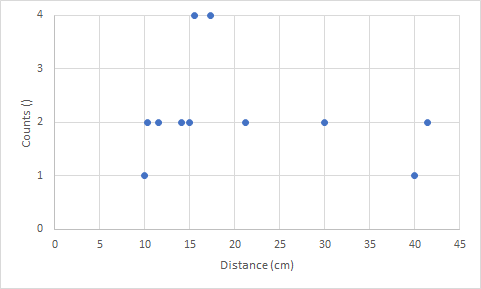
Now the effect for each of these groups of distances on the acoustic frequency response has to be calculated. Each of these groups of distances will produce a single sinus shaped deviation from a flat frequency response. For a visual representation please look at the pictures shown here Diffraction from baffle edges. When looking at the 12” cylindrical baffle in this link, you can clearly spot the sinus curve. When looking at the other pictures, you can also immediately spot that larger baffles give a higher frequent sinus curve in the diffraction pattern.
In the next step I calculate a sinus curve for each spot in the graph. I have to consider three things:
1. All curves have to have a minimum at 0 Hz,
2. the frequency is dependent on the distance and the speed of sound and
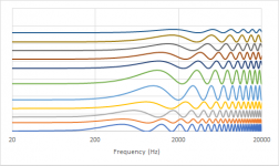
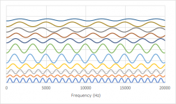
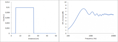
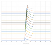
3. The amplitude is dependent on the abundance of each distance (= count). When calculating all these sinus curves individually, it will look like this. The sinus curve at the very bottom originates from the highest distance (41.41 cm).
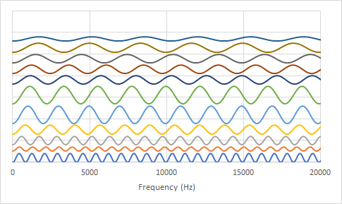
Now this is audio and it a common convention to plot the frequency axis not linearly but logarithmically.

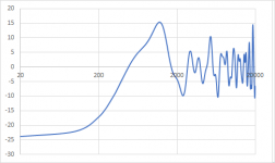
The total diffraction pattern can be seen when adding the curves.
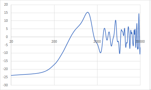
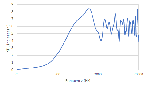
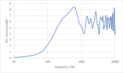
Now the scaling is a bit off. The x-axis is already fine since I considered the speed the sound when calculating Hz from cm but the y-axis is not. To fix this I have to discuss what this graph represents. To my understanding, this represents the additional sound pressure due to the half of the spherical wave which nominally is propagating to the back but is immediately reflected to the front due to the baffle, assuming an ideal point source and ideal reflectivity of the baffle. Since I used 24 points and calculated sinus curves ranging from -1 to 1 for each, the sum of them can now range from -24 to 24. -24 represents no reflection to the front (= just direct sound) whereas 24 represents full reflection to the front (= doubled sound pressure). By rescaling the reflections to range from 0 to 1 and adding the sound pressure from the direct sound, which is 1, I can calculate the sound pressure level increase when using just direct sound pressure as a reference.
Nevertheless, it seems I am wrong on this one and if someone can explain my mistake to me, I would be grateful. For a calculation giving the same results as The Edge I have to scale the reflected sound pressure to range from 0 to 2, meaning that the reflected sound pressure can be twice as high as the direct sound pressure. With this value I then do the same as previously described: I add 1 for the direct sound and calculate the sound pressure level using the direct sound pressure as reference.
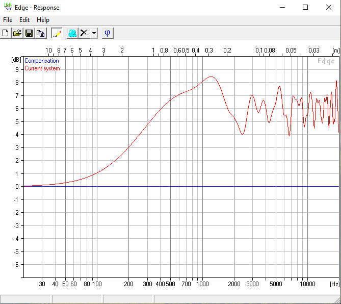
This then gives this plot, which looks very much like the result from The Edge.
I do see here quite regularly threads about diffraction but, respectfully, I have the impression that sometimes there is not enough understanding about diffractions. I am no expert either but I spent quite some time researching and simulating on this matter and I think I can share some thoughts which may be helpful.
I don’t want this thread to be about the fundamental physical background of diffractions, I don’t want it to be about the design of a specific cabinet and I also don’t aim to make a new tool to calculate diffractions. There are already plenty.
Instead it should be about a general understanding of cause and effect regarding diffractions. I want to describe what can be expected from different measures to tame diffractions for proper sound reproduction.
I already have to apologize here because this will become quite a wall of text but at least there will be some pictures.
How to calculate diffractions
For a better understanding I think it’s best to start to explain how software like The Edge simulates diffractions. I am not affiliated with the software in any way so I can’t say anything about the details, only how this works in general. The input for such a simulation may look like this.
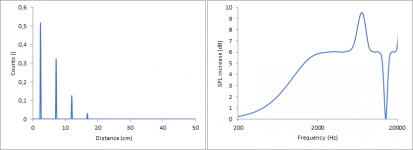
For each point at the edge of the baffle the software calculates the distance (Source –> Point at the baffle –> microphone) minus (Source –> microphone). For now, all my calculations will assume that the microphone is in infinite distance directly in front of the chassis. When doing exactly the same calculation in Excel, I get the following values as a function of the angle. I will call the result from this calculation “distance” from now on. 0° in this case is the perpendicular distance to the left edge and then every 15° there is another point at the edge in clockwise direction. It is quite easy to follow. The first 3 points are located at the left edge, each with slightly increasing distances, the next points are on top, which first decrease in distance until a distance of 10 cm is reached, representing the perpendicular distance to the top edge and so on. At an angle of about 270° three distances stand out representing the three points at the bottom edge.
This plot can now be rearranged, because for diffractions it does not matter under which angle which distance is obtained. Only the distances themselves matter. For symmetry reasons some of the distances are the same and they can then be summarized. For example, 15°, 165°, 195° and 345° all give 15.53 cm. To ease further calculations, I can group these 4 to a single data point with a higher weighted impact on the overall diffraction pattern. I do the same for all similar distances and get then the following graph.
Now the effect for each of these groups of distances on the acoustic frequency response has to be calculated. Each of these groups of distances will produce a single sinus shaped deviation from a flat frequency response. For a visual representation please look at the pictures shown here Diffraction from baffle edges. When looking at the 12” cylindrical baffle in this link, you can clearly spot the sinus curve. When looking at the other pictures, you can also immediately spot that larger baffles give a higher frequent sinus curve in the diffraction pattern.
In the next step I calculate a sinus curve for each spot in the graph. I have to consider three things:
1. All curves have to have a minimum at 0 Hz,
2. the frequency is dependent on the distance and the speed of sound and
3. The amplitude is dependent on the abundance of each distance (= count). When calculating all these sinus curves individually, it will look like this. The sinus curve at the very bottom originates from the highest distance (41.41 cm).
Now this is audio and it a common convention to plot the frequency axis not linearly but logarithmically.
The total diffraction pattern can be seen when adding the curves.
Now the scaling is a bit off. The x-axis is already fine since I considered the speed the sound when calculating Hz from cm but the y-axis is not. To fix this I have to discuss what this graph represents. To my understanding, this represents the additional sound pressure due to the half of the spherical wave which nominally is propagating to the back but is immediately reflected to the front due to the baffle, assuming an ideal point source and ideal reflectivity of the baffle. Since I used 24 points and calculated sinus curves ranging from -1 to 1 for each, the sum of them can now range from -24 to 24. -24 represents no reflection to the front (= just direct sound) whereas 24 represents full reflection to the front (= doubled sound pressure). By rescaling the reflections to range from 0 to 1 and adding the sound pressure from the direct sound, which is 1, I can calculate the sound pressure level increase when using just direct sound pressure as a reference.
Nevertheless, it seems I am wrong on this one and if someone can explain my mistake to me, I would be grateful. For a calculation giving the same results as The Edge I have to scale the reflected sound pressure to range from 0 to 2, meaning that the reflected sound pressure can be twice as high as the direct sound pressure. With this value I then do the same as previously described: I add 1 for the direct sound and calculate the sound pressure level using the direct sound pressure as reference.
This then gives this plot, which looks very much like the result from The Edge.
Attachments

The ideal baffle to minimize diffractions
What I did until now was adding up sinus curves with different frequencies and intensities. Mathematically speaking this is a Fourier transformation. The input it needs is a function which describes the intensity for each sinus curve (that’s what I called count) against the frequency for each curve (that’s what I called distance). So, the necessary data for a Fourier transformation is actually in the 3rd picture in this post. For the purpose of diffractions, it is not necessary to know a lot about Fourier transformations, but most importantly: they can be reversed. This means you can choose your desired diffraction pattern and the Fourier transformation will give you a hint what has to be done to achieve it.
Ideally, in a dream world, the diffraction pattern would not show a baffle step and it would not show any deviations from a flat line. Previously I said that each sinus curve will have a minimum at 0 Hz. This means as long as you sum ANY sinus curves, which is the same as using ANY baffle, there will be this minimum at 0 Hz. It is not possible to add some magical baffle shape which will get rid of it. You can move the step to lower frequencies, yes, but you cannot get rid of it completely.
The wet dream of diffractions is not possible. What is the second-best solution? A smooth baffle step followed by a completely flat line.
To get to an actual baffle behaving ideally, two steps are required. First, a Fourier transformation has to be applied to the ideal diffraction pattern and then a baffle has to be manually adopted giving the same count vs distance graph obtained from the Fourier transformation. Starting with the first step, I tried to find out how different graph vs distance curves affect the diffraction pattern. I used some curves and did Fourier transformations on them.
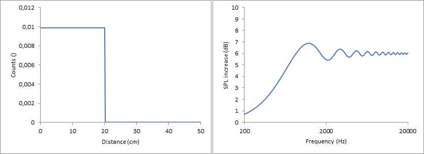
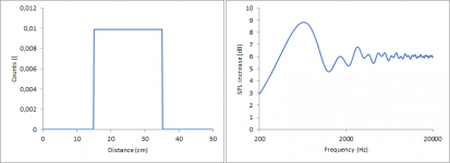
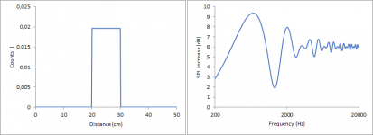
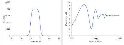
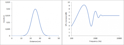
In each case from now on the left graph represents the baffle. The right graph represents the diffraction pattern such a baffle would give.
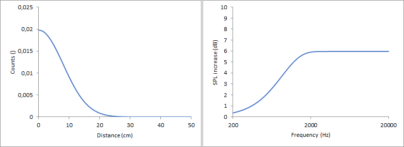
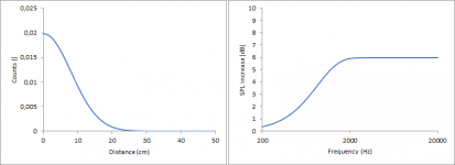
Gaussian, maximum at 0 cm
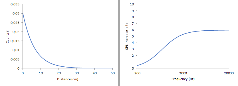
Exponential Decay
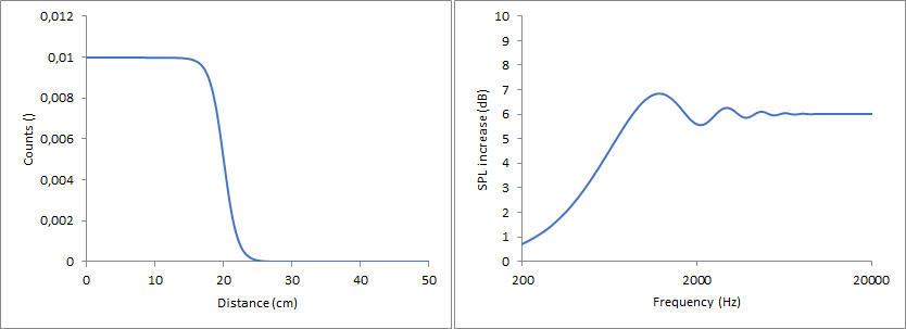
Sigmoid function, turning point at 20 cm
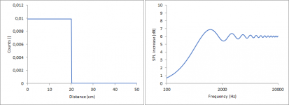
Rectangular signal, transition at 20 cm
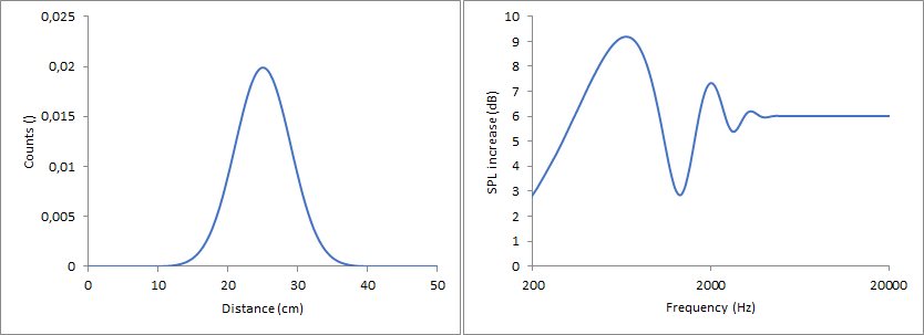
Gaussian, maximum at 25 cm
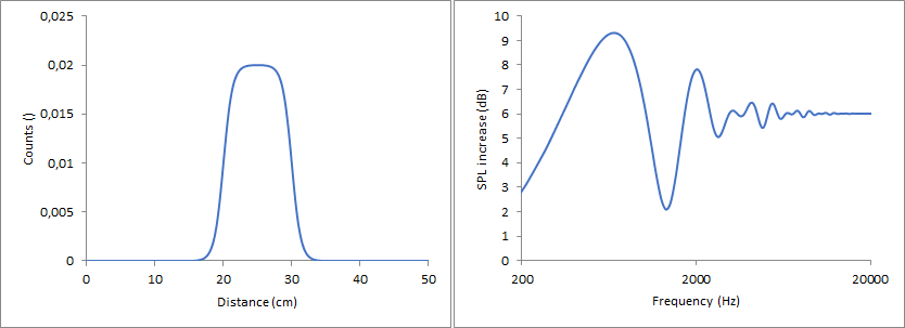
Sigmoid function, turning points at 20 and 30 cm
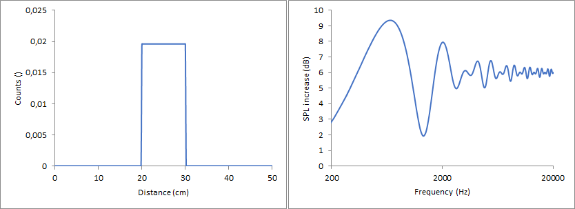
Rectangular function, transitions at 20 and 30 cm
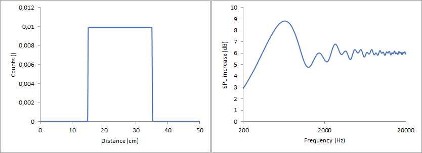
Rectangular function, transitions at 15 and 35 cm

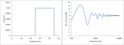
Rectangular function, transitions at 22.5 and 27.5 cm
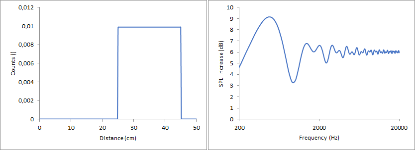
Rectangular function, transitions at 25 and 45 cm
What I did until now was adding up sinus curves with different frequencies and intensities. Mathematically speaking this is a Fourier transformation. The input it needs is a function which describes the intensity for each sinus curve (that’s what I called count) against the frequency for each curve (that’s what I called distance). So, the necessary data for a Fourier transformation is actually in the 3rd picture in this post. For the purpose of diffractions, it is not necessary to know a lot about Fourier transformations, but most importantly: they can be reversed. This means you can choose your desired diffraction pattern and the Fourier transformation will give you a hint what has to be done to achieve it.
Ideally, in a dream world, the diffraction pattern would not show a baffle step and it would not show any deviations from a flat line. Previously I said that each sinus curve will have a minimum at 0 Hz. This means as long as you sum ANY sinus curves, which is the same as using ANY baffle, there will be this minimum at 0 Hz. It is not possible to add some magical baffle shape which will get rid of it. You can move the step to lower frequencies, yes, but you cannot get rid of it completely.
The wet dream of diffractions is not possible. What is the second-best solution? A smooth baffle step followed by a completely flat line.
To get to an actual baffle behaving ideally, two steps are required. First, a Fourier transformation has to be applied to the ideal diffraction pattern and then a baffle has to be manually adopted giving the same count vs distance graph obtained from the Fourier transformation. Starting with the first step, I tried to find out how different graph vs distance curves affect the diffraction pattern. I used some curves and did Fourier transformations on them.
In each case from now on the left graph represents the baffle. The right graph represents the diffraction pattern such a baffle would give.
Gaussian, maximum at 0 cm
Exponential Decay
Sigmoid function, turning point at 20 cm
Rectangular signal, transition at 20 cm
Gaussian, maximum at 25 cm
Sigmoid function, turning points at 20 and 30 cm
Rectangular function, transitions at 20 and 30 cm
Rectangular function, transitions at 15 and 35 cm
Rectangular function, transitions at 22.5 and 27.5 cm
Rectangular function, transitions at 25 and 45 cm
Attachments
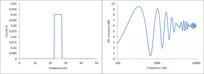


Rectangular function, transitions at 5 and 25 cm
From these curves some qualitative observations can be made.
- It can be seen that a smooth diffraction pattern can only be achieved when you have a lot of small distances followed by a steady decrease towards higher distances.
- A lack of small distances will mess up the lower frequencies.
- A smooth transition from a high count of distances to a low count of distances will smooth out the higher frequencies. The shape of the transition does change the pattern a bit but isn’t super important.
- It is beneficial to spread out the distances over a wide range instead of a sharp distribution.
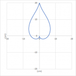
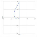
The ideal diffraction pattern can be obtained with a baffle following a gaussian in the count vs distance graph. Now for the second step: getting a baffle which corresponds to the chosen count vs distance graph. A flat baffle producing a Gaussian curve is very much achievable although not very easy to build. It would look like either of those drawings with the chassis at x=0, y=0 in each case. I cut it off at a maximum distance of 20 cm, but it would expand further. You get the idea. For the purpose of diffractions on axis all three drawings are identical and you could list infinite more of them.
Baffles with gaussian diffraction profile
One could also go for a three-dimensional shape. In this case something like a paraboloid or a two-sheeted hyperboloid is probably close to ideal with the chassis at the tip. Most noteworthy, they probably would both outperform a sphere, since a sphere lacks the long distances.
Attachments
Diffraction of a rectangular baffle
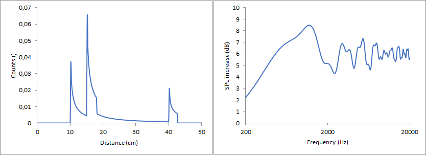
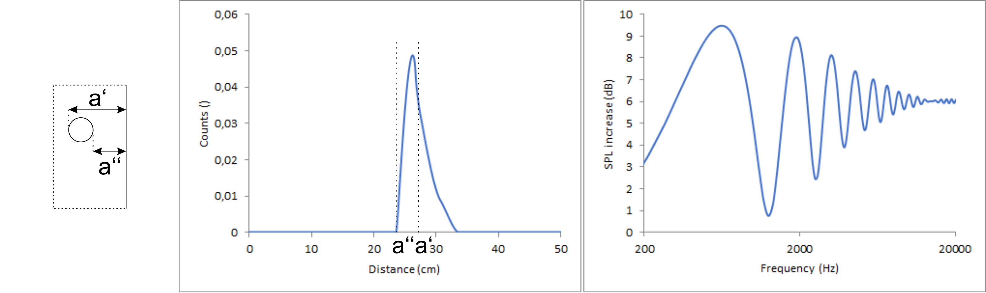
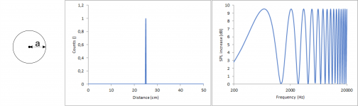
While those shapes certainly look interesting, they are not convenient. Much more relevant in practice is to find a way to shape a rectangular baffle to come as close to the gaussian as possible. So, lets analyse the count vs distance graphs of a rectangular baffle. The starting point for this is a single, straight, infinite edge in a distance of 25 cm to an ideal point source. For this setup the count vs. distance graph looks like this:
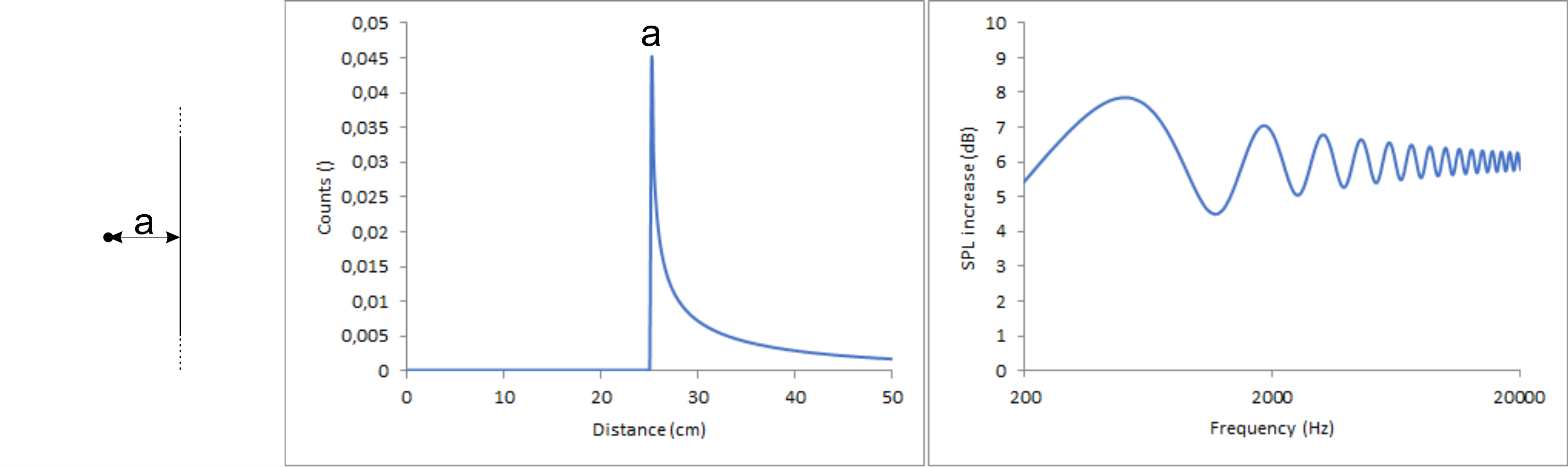
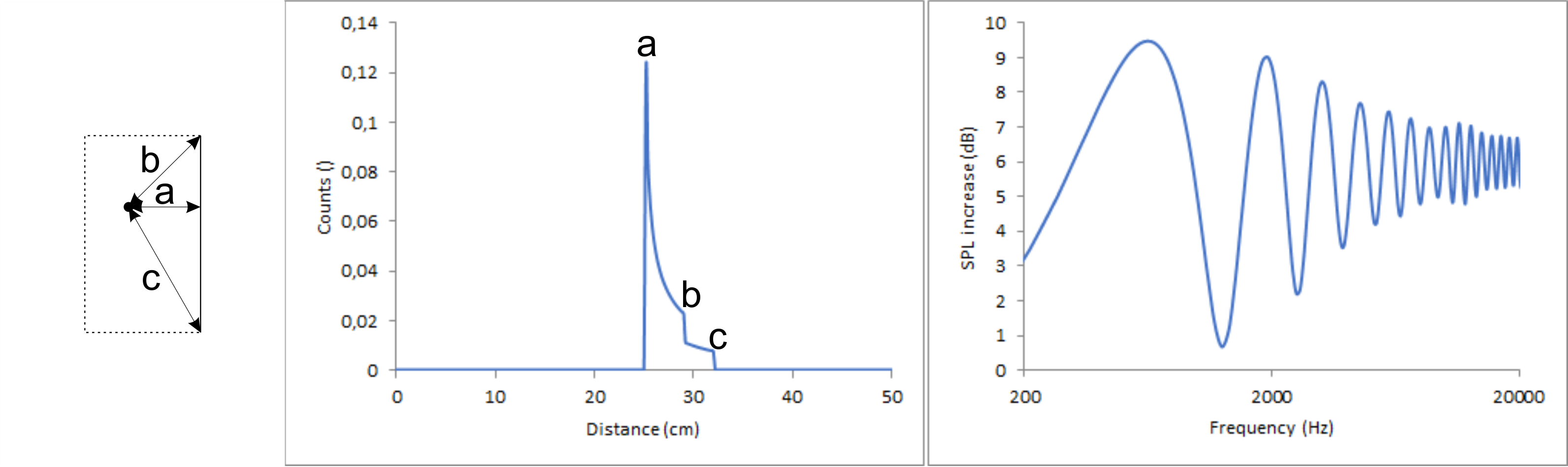
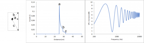
One can clearly see the perpendicular distance a in the count vs distance drawing. In a real box you don’t have infinite edges but each is limited at two different points represented by the bordering edges. When adding this to the equation, the baffle is altered as shown in the following drawing.
Let me show you for comparison the calculated diffraction pattern if not a straight edge but a cylinder was simulated with a radius of 25 cm.
When comparing the last two diffraction patterns, the position of the maxima and minima is the same in both drawings but for a straight, finite edge the pattern converges to 6 dB with higher frequencies, while the amplitude for the cylinder stays the same over the whole frequency range. This is an important point because this means qualitatively a single edge with a perpendicular distance a and a single distance a behave the same but for the straight edge you only have to focus on the low frequency part. As a consequence, the low frequency part of a rectangular baffle can be described qualitatively in good approximation by using just the four rectangular distances, calculating four corresponding sinus curves from them. The high frequency part will in the end always be decent.
When combining four edges to a full baffle, the relative intensities of these edges have to be discussed. Since sounds propagates in each direction equally, each direction from the source to an edge has to be weighted equally. When deviating from a perpendicular distance by a small angle, each distance increases by the same factor, meaning that in absolute numbers a small distance increases less than a larger one. This results in edges further away from the chassis producing smaller spikes in the count vs distance graph.
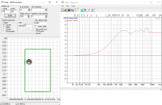
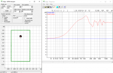
With this model at hand, I recalculated the baffle initially used in The Edge. Since I am using now a continuous curve and no longer just 24 points, I also cranked up the number of points in The Edge to the maximum. You can clearly see that the results are the same and therefore my model is still correct.

Influence of chassis dimensions, bevelled and rounded edges
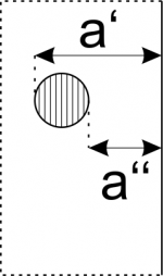
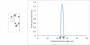
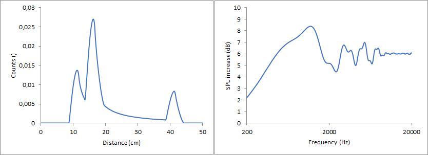
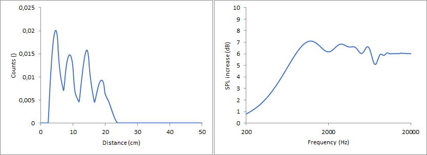
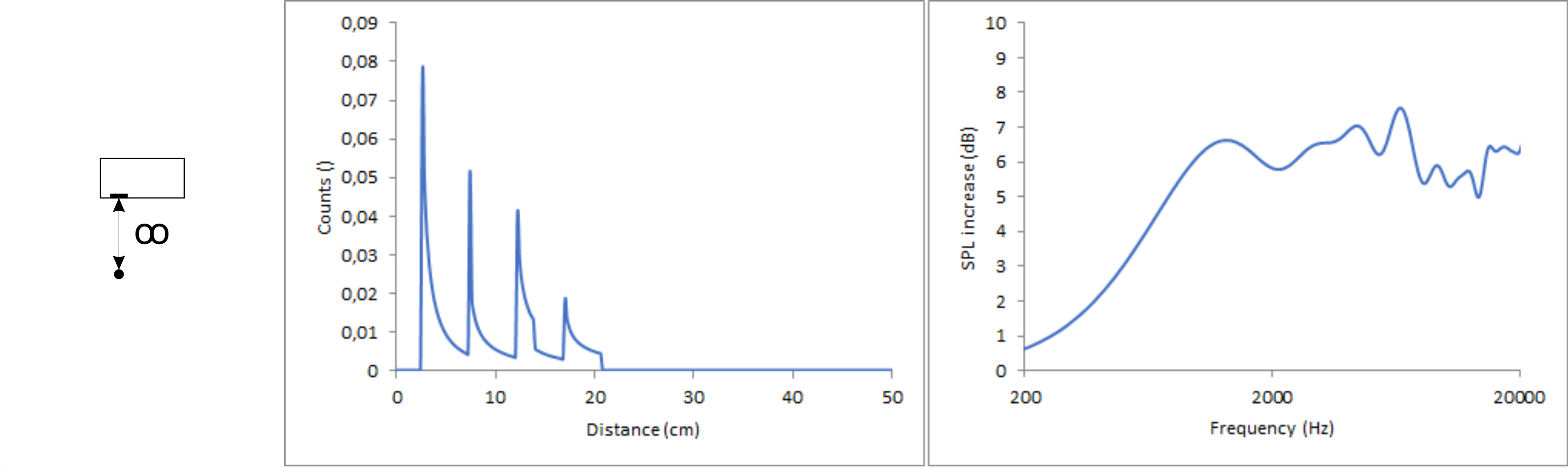
Until now I assumed an ideal point-source. There is no such thing in reality. In reality each source has a finite size. However, it seems to be a good approximation to assume that each individual spot on the source can be regarded as a single ideal point source, ultimately forming an array of point-sources. When plotting the density of the point sources as a function of the perpendicular distance to a finite edge, the following graph is obtained.
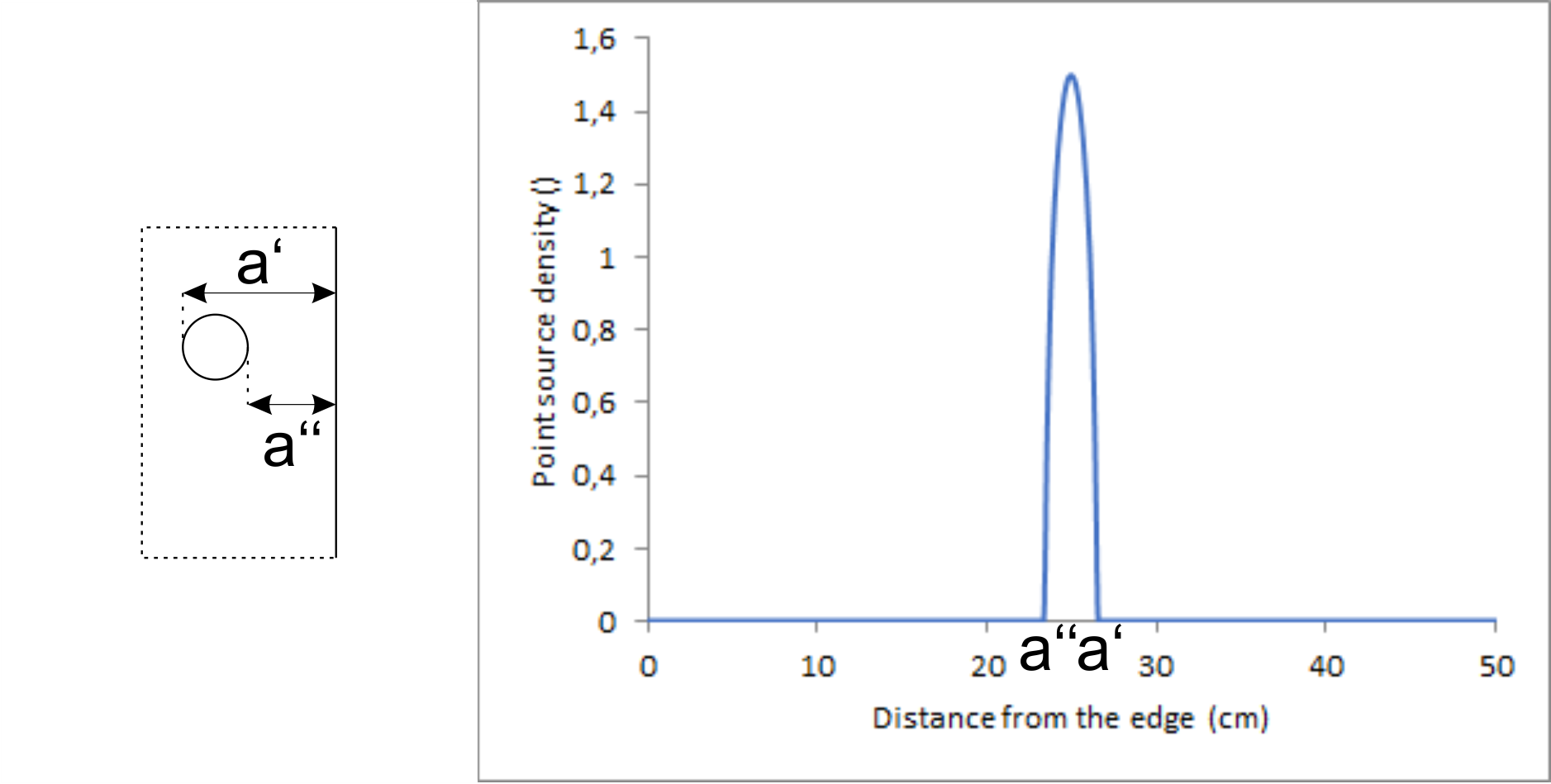
To calculate the overall diffraction pattern for the shown arrangement, I divided the chassis in several lines. For any point on the same line the perpendicular distance to the edge is the same. Therefore, I can use a single "edge shape" to describe a single line. But on a single line the upper and lower limits to the bordering edges differ depending on the actual point in question. To take this into account, both limits had to be replaced by linear decays instead of discontinuities. The linear decays are calculated in a way to consider the length of the line and the overall geometry. Each "edge shape" has then to be weighted according to the point source density shown in the previous picture.

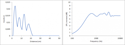
The calculated "edge shapes" for each individual line are shown in the following picture.
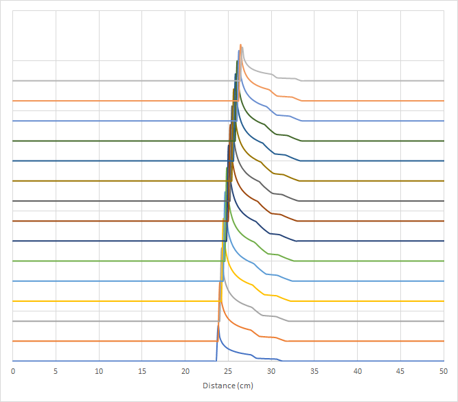
These curves can be summed giving the overall count vs distance graph for a source with finite dimension and can further be transformed to give the diffraction pattern.
Qualitatively this curve can again be described as a single sinus curve corresponding to a single distance with decreasing deviation from 6 dB with increasing frequency. It is somewhat similar to the gaussian at a distance of 25 cm to the point source shown earlier. When evaluating the maxima and minima in the diffraction pattern, the dominant frequency corresponds pretty precisely to an edge in a distance a.
In other words, this kind of smoothening of the diffraction pattern is beaming.
While those shapes certainly look interesting, they are not convenient. Much more relevant in practice is to find a way to shape a rectangular baffle to come as close to the gaussian as possible. So, lets analyse the count vs distance graphs of a rectangular baffle. The starting point for this is a single, straight, infinite edge in a distance of 25 cm to an ideal point source. For this setup the count vs. distance graph looks like this:
One can clearly see the perpendicular distance a in the count vs distance drawing. In a real box you don’t have infinite edges but each is limited at two different points represented by the bordering edges. When adding this to the equation, the baffle is altered as shown in the following drawing.
Let me show you for comparison the calculated diffraction pattern if not a straight edge but a cylinder was simulated with a radius of 25 cm.
When comparing the last two diffraction patterns, the position of the maxima and minima is the same in both drawings but for a straight, finite edge the pattern converges to 6 dB with higher frequencies, while the amplitude for the cylinder stays the same over the whole frequency range. This is an important point because this means qualitatively a single edge with a perpendicular distance a and a single distance a behave the same but for the straight edge you only have to focus on the low frequency part. As a consequence, the low frequency part of a rectangular baffle can be described qualitatively in good approximation by using just the four rectangular distances, calculating four corresponding sinus curves from them. The high frequency part will in the end always be decent.
When combining four edges to a full baffle, the relative intensities of these edges have to be discussed. Since sounds propagates in each direction equally, each direction from the source to an edge has to be weighted equally. When deviating from a perpendicular distance by a small angle, each distance increases by the same factor, meaning that in absolute numbers a small distance increases less than a larger one. This results in edges further away from the chassis producing smaller spikes in the count vs distance graph.
With this model at hand, I recalculated the baffle initially used in The Edge. Since I am using now a continuous curve and no longer just 24 points, I also cranked up the number of points in The Edge to the maximum. You can clearly see that the results are the same and therefore my model is still correct.
Influence of chassis dimensions, bevelled and rounded edges
Until now I assumed an ideal point-source. There is no such thing in reality. In reality each source has a finite size. However, it seems to be a good approximation to assume that each individual spot on the source can be regarded as a single ideal point source, ultimately forming an array of point-sources. When plotting the density of the point sources as a function of the perpendicular distance to a finite edge, the following graph is obtained.
To calculate the overall diffraction pattern for the shown arrangement, I divided the chassis in several lines. For any point on the same line the perpendicular distance to the edge is the same. Therefore, I can use a single "edge shape" to describe a single line. But on a single line the upper and lower limits to the bordering edges differ depending on the actual point in question. To take this into account, both limits had to be replaced by linear decays instead of discontinuities. The linear decays are calculated in a way to consider the length of the line and the overall geometry. Each "edge shape" has then to be weighted according to the point source density shown in the previous picture.
The calculated "edge shapes" for each individual line are shown in the following picture.
These curves can be summed giving the overall count vs distance graph for a source with finite dimension and can further be transformed to give the diffraction pattern.
Qualitatively this curve can again be described as a single sinus curve corresponding to a single distance with decreasing deviation from 6 dB with increasing frequency. It is somewhat similar to the gaussian at a distance of 25 cm to the point source shown earlier. When evaluating the maxima and minima in the diffraction pattern, the dominant frequency corresponds pretty precisely to an edge in a distance a.
In other words, this kind of smoothening of the diffraction pattern is beaming.
Attachments


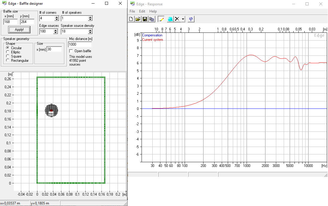
I made another comparison between my model in Excel and a baffle calculated in The Edge. I am using the same dimensions as before but this time with a 30 mm source. They look, again, the same.
 In the next step I want to show the influences of bevelled edges. Sadly, I couldn’t find information on how the angle at the edge influences the intensity of a diffraction, so the exact numbers are pretty much only guesswork. On the other hand, the distances resulting from certain baffle shapes can be calculated easily, so they are most certainly correct. Still, I would be happy if someone could point me in the right direction on this one.
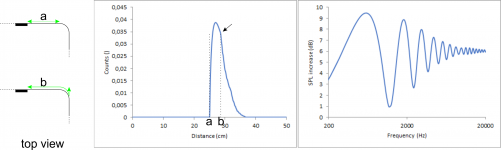
To better show the impact of bevelled edges, I will use a single point source again. A bevelled edge consists basically just of two consecutive edges with, to my understanding, different impact on the diffraction pattern. The first edge is hit be the full spherical wave but its angle is less than 90°, so it should have less impact than a regular 90° edge. The second edge is again less than 90° and it is only hit by the part diffracted by the first edge. Therefore, it should be even weaker than the first edge.
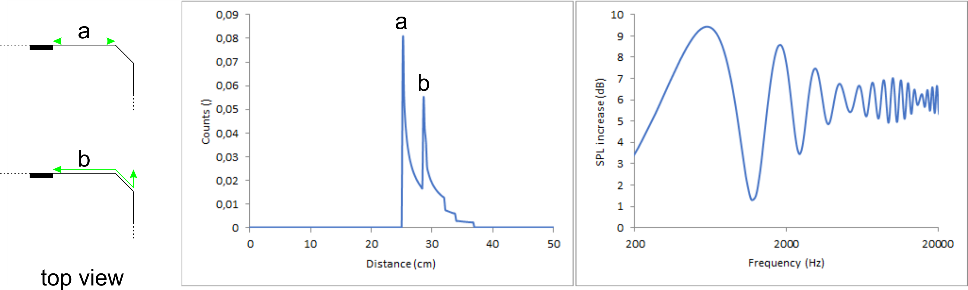 Qualitatively, it is an overlay of two sinus curves with slightly different frequency resulting in a beat. Please note that for a just the distance along the baffle has to be covered but for b first the way along the baffle, then along the bevelled edge and finally the way back to the plane of the baffle has to be considered. That is the additional way the sound has to take assuming a listener directly in front of the speaker in infinite distance.
As a sidenote: If the edges of the speaker are not parallel, they will still produce the same diffraction pattern since only the shortest distance to each edge count, not the direction in which this distance is reached. With non-parallel edges each edge will still only have a single shortest distance to the point source.
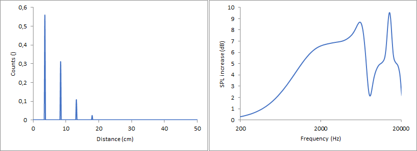
Based on my assumptions for bevelled edges, a rounded edge behaves like infinite, small, consecutive edges. By the same logic used for bevelled edges, it will then give the following diffraction pattern. I calculated it in a similar way as I did when calculating a source with finite dimensions. I used an exponential decay ranging from a to b and at each point of the decay I started a weighted “edge shape” with adjusted limits representing the bordering edges. Then I summed these curves.
 Overall, the influence of this curve on the diffraction pattern can again best be described as a single sinus curve smoothened out to higher frequencies. When evaluating just the maxima and minima in the diffraction pattern, the dominant frequency is somewhere between a and b. In fact, it is relatively close to the distance a+r with r being the radius of the rounded edge. For completeness: b=a+r*(1+(pi/2)). This means when building a cabinet with a certain diffraction pattern and adding rounded edges later with a router will barely change the position of peaks in the diffraction pattern, it will mainly reduce the intensity of those deviations, most efficiently at high frequencies.
One can immediately see the resemblance with the results obtained from a source with finite dimensions on a baffle with untreated edges. Qualitatively speaking, it barely matters if you add rounded edges or increase the size of the chassis diffraction wise.
A realistic baffle with minimal diffractions
The next challenge is to use the presented tools to get something close to a gaussian in the count vs distance graph but with a rectangular baffle.
In the previous part I have shown that whatever you do, bevelled edges, rounded edges or a larger chassis, qualitatively you will always stick with one (or two in case of bevelled edges) sinus curves in the diffraction pattern for each edge converging to 6 dB at higher frequencies. In order to optimize the whole baffle, it is therefore enough to think about a way how to arrange 4 (or up to 8) sinus curves in a way that the low frequency part gives a flat line at 6 dB.
What’s needed for this, is the same distribution also used for square waves (Rechteckschwingung – Wikipedia). You will notice in this picture that for square waves the phase is shifted so that all curves all start at 0, for diffractions the curves have to start at a minimum. When using the required phase shift, the diffraction pattern will look like in the following picture. In this graph the first distance is set to 2.4 cm, the next to 7.2 cm (=2.4+1*4.8), the next one to 12 cm (=2.4+2*4.8) and the final one to 16.8 cm (=2.4+3*4.8).
 This graph actually looks very good. First there is a baffle step, then there is a flat part which is at 6 dB and finally there is a single undesired maximum followed by a minimum.
I want to stress that these extrema are the price you have to pay for the smooth behaviour at lower frequencies. Since there are ways to address issues in the high frequency region but there are none for the low frequency region, it is a perfectly fine price to pay.
The position of the peaks is defined by the distance between the 4 input distances. In this case it is at 7100 Hz which corresponds to a wavelength of 4.8 cm. The closer the distances in the count vs distance graph are, the higher the frequency of the peak in the diffraction pattern. Regarding edge treatment I have two choices. Either I use bevelled edges designed in a way so that I ultimately end up with 8 peaks in the count vs distance graph, all equally spread out to shift the unwanted peaks up to higher frequencies no longer within hearing range. Or I use rounded edges smoothening out the high frequency part so that the peak becomes much smaller. Either way, a finite source size and the behaviour of straight edges in general will greatly reduce the unwanted peak even further.
So, these are the ideal proportions. Let’s use them to calculate an actual rectangular baffle with a 30 mm source, once in Excel and once in The Edge.

 The minimum completely disappeared and the maximum is greatly reduced in intensity. Overall, this arrangement gives a deviation of about 1.5 dB over the range from 1 kHz to 20 kHz before edge treatment is applied.
This is, without a doubt, the ideal arrangement when optimizing the whole range, however, some adjustments can be made when considering that all these calculations focus primarily on the tweeter and the tweeter probably doesn’t need a flat line down to 1 kHz. When using again equally spaced input peaks in an interval of 4.8 cm but this time not starting at 2.4 cm but at 3.6 cm the following curve is obtained.
 The differences to the previous approach are:
- the flat part around 2 kHz is now slightly above 6 dB.
- the first maximum is split up in a maximum which is at lower frequencies and a minimum which is at higher frequencies. The maximum is weaker so it should be less of an issue and the minimum is at higher frequencies so it can be better addressed by other means.
Whatever happens beyond the first minimum can safely be ignored in all considerations. An actual baffle based on this will look like this.
 As expected, the low frequency part as a whole is now slightly above 6 dB but the maximum at about 6 kHz is less of an issue whereas the minimum at 7.5 kHz is at a higher frequency and can therefore be better addressed with edge treatment. I am not sure if it is actually better diffraction wise since the deviations no longer are within 1.5 dB but at about 2 dB. However, from a handyman point of view, this one is probably easier to incorporate in a project since the tweeter is no longer so closely hugging the left edge.
Either way, both examples are super similar not in their actual dimensions but regarding their theoretical background.
To better show the impact of bevelled edges, I will use a single point source again. A bevelled edge consists basically just of two consecutive edges with, to my understanding, different impact on the diffraction pattern. The first edge is hit be the full spherical wave but its angle is less than 90°, so it should have less impact than a regular 90° edge. The second edge is again less than 90° and it is only hit by the part diffracted by the first edge. Therefore, it should be even weaker than the first edge.
As a sidenote: If the edges of the speaker are not parallel, they will still produce the same diffraction pattern since only the shortest distance to each edge count, not the direction in which this distance is reached. With non-parallel edges each edge will still only have a single shortest distance to the point source.
Based on my assumptions for bevelled edges, a rounded edge behaves like infinite, small, consecutive edges. By the same logic used for bevelled edges, it will then give the following diffraction pattern. I calculated it in a similar way as I did when calculating a source with finite dimensions. I used an exponential decay ranging from a to b and at each point of the decay I started a weighted “edge shape” with adjusted limits representing the bordering edges. Then I summed these curves.
One can immediately see the resemblance with the results obtained from a source with finite dimensions on a baffle with untreated edges. Qualitatively speaking, it barely matters if you add rounded edges or increase the size of the chassis diffraction wise.
A realistic baffle with minimal diffractions
The next challenge is to use the presented tools to get something close to a gaussian in the count vs distance graph but with a rectangular baffle.
In the previous part I have shown that whatever you do, bevelled edges, rounded edges or a larger chassis, qualitatively you will always stick with one (or two in case of bevelled edges) sinus curves in the diffraction pattern for each edge converging to 6 dB at higher frequencies. In order to optimize the whole baffle, it is therefore enough to think about a way how to arrange 4 (or up to 8) sinus curves in a way that the low frequency part gives a flat line at 6 dB.
What’s needed for this, is the same distribution also used for square waves (Rechteckschwingung – Wikipedia). You will notice in this picture that for square waves the phase is shifted so that all curves all start at 0, for diffractions the curves have to start at a minimum. When using the required phase shift, the diffraction pattern will look like in the following picture. In this graph the first distance is set to 2.4 cm, the next to 7.2 cm (=2.4+1*4.8), the next one to 12 cm (=2.4+2*4.8) and the final one to 16.8 cm (=2.4+3*4.8).
I want to stress that these extrema are the price you have to pay for the smooth behaviour at lower frequencies. Since there are ways to address issues in the high frequency region but there are none for the low frequency region, it is a perfectly fine price to pay.
The position of the peaks is defined by the distance between the 4 input distances. In this case it is at 7100 Hz which corresponds to a wavelength of 4.8 cm. The closer the distances in the count vs distance graph are, the higher the frequency of the peak in the diffraction pattern. Regarding edge treatment I have two choices. Either I use bevelled edges designed in a way so that I ultimately end up with 8 peaks in the count vs distance graph, all equally spread out to shift the unwanted peaks up to higher frequencies no longer within hearing range. Or I use rounded edges smoothening out the high frequency part so that the peak becomes much smaller. Either way, a finite source size and the behaviour of straight edges in general will greatly reduce the unwanted peak even further.
So, these are the ideal proportions. Let’s use them to calculate an actual rectangular baffle with a 30 mm source, once in Excel and once in The Edge.
This is, without a doubt, the ideal arrangement when optimizing the whole range, however, some adjustments can be made when considering that all these calculations focus primarily on the tweeter and the tweeter probably doesn’t need a flat line down to 1 kHz. When using again equally spaced input peaks in an interval of 4.8 cm but this time not starting at 2.4 cm but at 3.6 cm the following curve is obtained.
- the flat part around 2 kHz is now slightly above 6 dB.
- the first maximum is split up in a maximum which is at lower frequencies and a minimum which is at higher frequencies. The maximum is weaker so it should be less of an issue and the minimum is at higher frequencies so it can be better addressed by other means.
Whatever happens beyond the first minimum can safely be ignored in all considerations. An actual baffle based on this will look like this.
Either way, both examples are super similar not in their actual dimensions but regarding their theoretical background.
Attachments


Spatial changes of diffraction patterns
Until now all calculations done here only consider the diffraction pattern produced at a single point in space which, obviously, should be the listening position. I assumed that this point is straight in front of the speaker and in an infinite distance. That’s not realistic, so let’s choose something different.
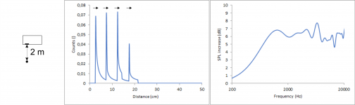
To show the influence of the distance between listener and chassis I did two calculations. Both use the same baffle with 2.4/7.2/12/16.8 cm perpendicular distances to the edges which I already used before and an ideal point source. In one calculation the listener is in infinite distance to the chassis, in the other he is at 2 m.
 When moving the listener closer all perpendicular distances to the edges get slightly larger but they do it somewhat evenly so overall, they are still spread out pretty much as before. For this purpose, 2 m is still pretty much the same as an infinite distance when keeping in mind that the dimensions of the baffle are in the cm range. Getting closer doesn’t change a lot.
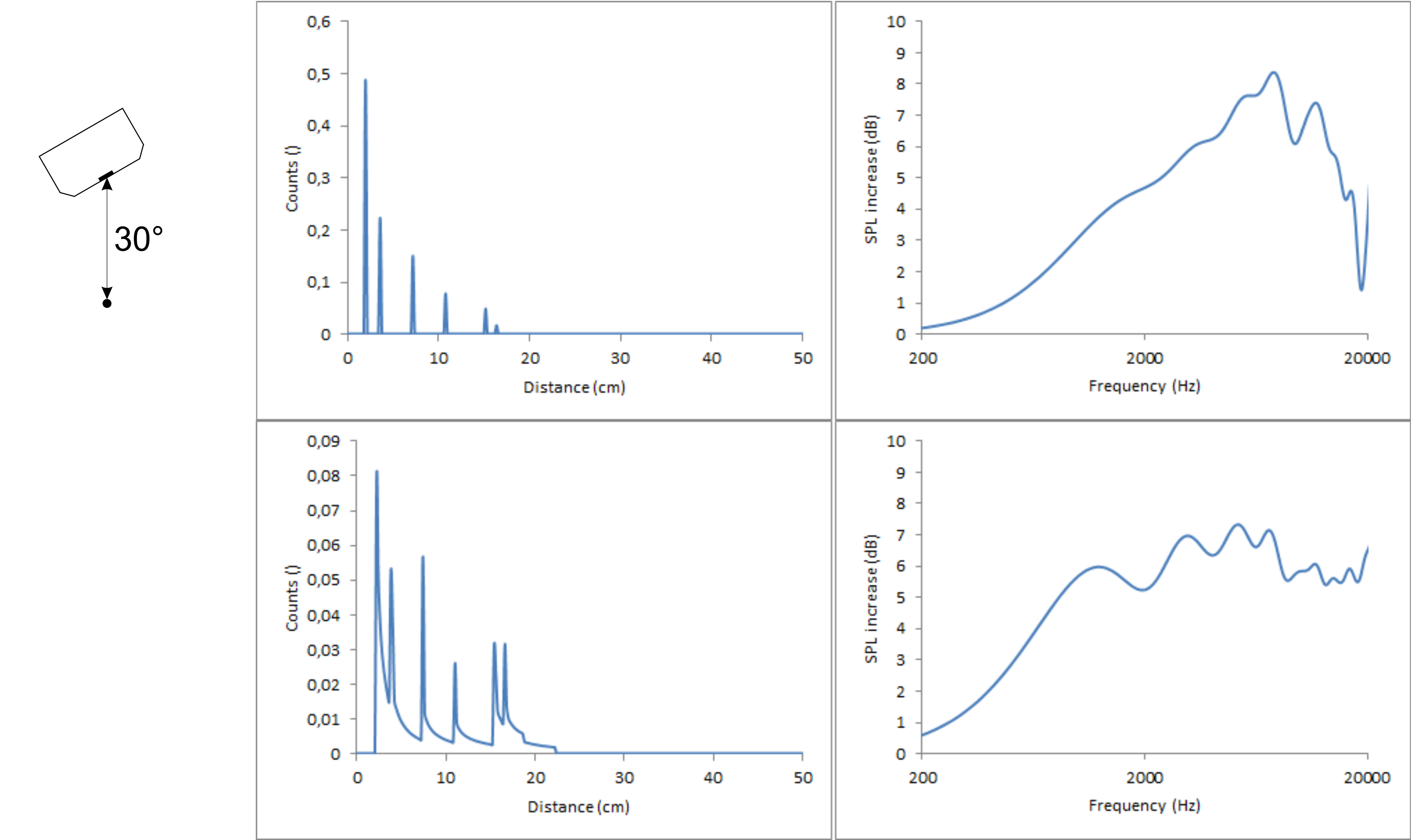
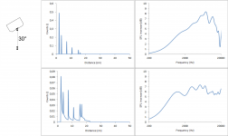
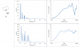
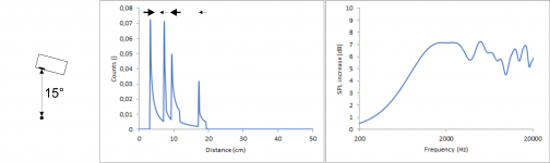
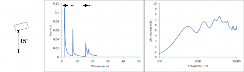
It is a different story when tilting the speakers. This messes up the diffraction pattern big time. To show this, I did two calculation with a distance of 2 m between chassis and listener and a baffle with 2.4/7.2/12/16.8 cm perpendicular distances each tilted by 15°, once moving the 2.4 cm edge closer to the listener and once moving the 12 cm edge closer to the listener.

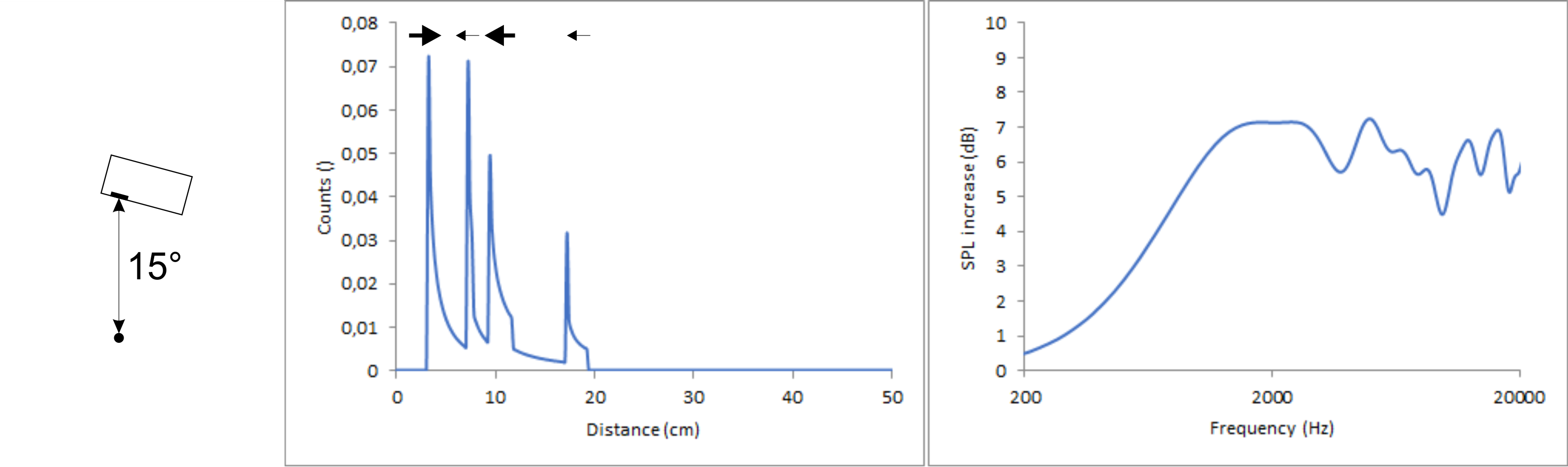 The distances to the top (second peak) and to the bottom (fourth peak) both get slightly smaller because the points at the edges where these shortest distances are, move slightly closer to the listener. Those points only depend on the angle the speaker is tilted, not on the direction of the tilt. The small distance to the left (first peak) gets smaller (first figure) or larger (second figure) by a “significant” factor but since the distance is small to begin with, this factor has only minor impact in absolute terms. The real deal breaker is the distance to the right (third peak). It is also multiplied with a significant factor but this time the original distance is already quite large. Therefore, it is shifted by quite a lot in both cases.
Unfortunately, this means that it is not possible to get ideal diffraction behaviour on- and off-axis simultaneously in the horizontal plane using just a flat, rectangular baffle if either distance left or right is large. The best diffraction behaviour in the horizontal plane, while maintaining the equally spread out distances edges in the count vs distance graph can be achieved if the shortest and second shortest distances are left and right, while the largest and second largest distances are top and bottom, very much like a D’Appolito arrangement.
To improve the diffraction behaviour off-axis, rounded and bevelled edges can help quite a lot. Bevelled edges are basically just two consecutive edges with, so I assume, less pronounced diffractions due to the smaller than 90° angle. So when going for equally spaced distances on-axis, one could use the distance to the top (no bevelled edge) as the smallest distance, the distance left and right (bevelled edge) to the first edge as the second smallest distance, the distance left and right to the rear end of the bevelled edge as the third smallest distance and bottom could be used as the largest distance. This way, when tilting the speaker, the distances left and right will split and while they are no longer equally spread, at least they don’t cluster too much.
Similar thing can be achieved with a generous rounding left and right.
Influence of the baffle material
In all my considerations I assumed ideal behaviour of the baffle itself. That is ideal reflectivity for sound. As a reminder, diffractions occur due to reflections of the formally backwards propagating halfwave which is immediately reflected back forward. If the reflectivity of the baffle decreases, the diffraction pattern will converge to 0 dB. This can happen due to surface treatment of the baffle but it also happens naturally to some degree.
Until now all calculations done here only consider the diffraction pattern produced at a single point in space which, obviously, should be the listening position. I assumed that this point is straight in front of the speaker and in an infinite distance. That’s not realistic, so let’s choose something different.
To show the influence of the distance between listener and chassis I did two calculations. Both use the same baffle with 2.4/7.2/12/16.8 cm perpendicular distances to the edges which I already used before and an ideal point source. In one calculation the listener is in infinite distance to the chassis, in the other he is at 2 m.
It is a different story when tilting the speakers. This messes up the diffraction pattern big time. To show this, I did two calculation with a distance of 2 m between chassis and listener and a baffle with 2.4/7.2/12/16.8 cm perpendicular distances each tilted by 15°, once moving the 2.4 cm edge closer to the listener and once moving the 12 cm edge closer to the listener.
Unfortunately, this means that it is not possible to get ideal diffraction behaviour on- and off-axis simultaneously in the horizontal plane using just a flat, rectangular baffle if either distance left or right is large. The best diffraction behaviour in the horizontal plane, while maintaining the equally spread out distances edges in the count vs distance graph can be achieved if the shortest and second shortest distances are left and right, while the largest and second largest distances are top and bottom, very much like a D’Appolito arrangement.
To improve the diffraction behaviour off-axis, rounded and bevelled edges can help quite a lot. Bevelled edges are basically just two consecutive edges with, so I assume, less pronounced diffractions due to the smaller than 90° angle. So when going for equally spaced distances on-axis, one could use the distance to the top (no bevelled edge) as the smallest distance, the distance left and right (bevelled edge) to the first edge as the second smallest distance, the distance left and right to the rear end of the bevelled edge as the third smallest distance and bottom could be used as the largest distance. This way, when tilting the speaker, the distances left and right will split and while they are no longer equally spread, at least they don’t cluster too much.
Similar thing can be achieved with a generous rounding left and right.
Influence of the baffle material
In all my considerations I assumed ideal behaviour of the baffle itself. That is ideal reflectivity for sound. As a reminder, diffractions occur due to reflections of the formally backwards propagating halfwave which is immediately reflected back forward. If the reflectivity of the baffle decreases, the diffraction pattern will converge to 0 dB. This can happen due to surface treatment of the baffle but it also happens naturally to some degree.
Attachments

-very nice!
However, a thread is a poor "format" of this information. Instead turn it into an article for the forum (..but keep this thread for the initial responses.)
diyAudio - Article
Audioholics might also like this as an article:
Loudspeaker Design, Measurements, Theory | Audioholics
However, a thread is a poor "format" of this information. Instead turn it into an article for the forum (..but keep this thread for the initial responses.)
diyAudio - Article
Audioholics might also like this as an article:
Loudspeaker Design, Measurements, Theory | Audioholics
Last edited:
It is a different story when tilting the speakers.
How about some really heavy tilt? Like in case of Shahinian or Heed speakers?

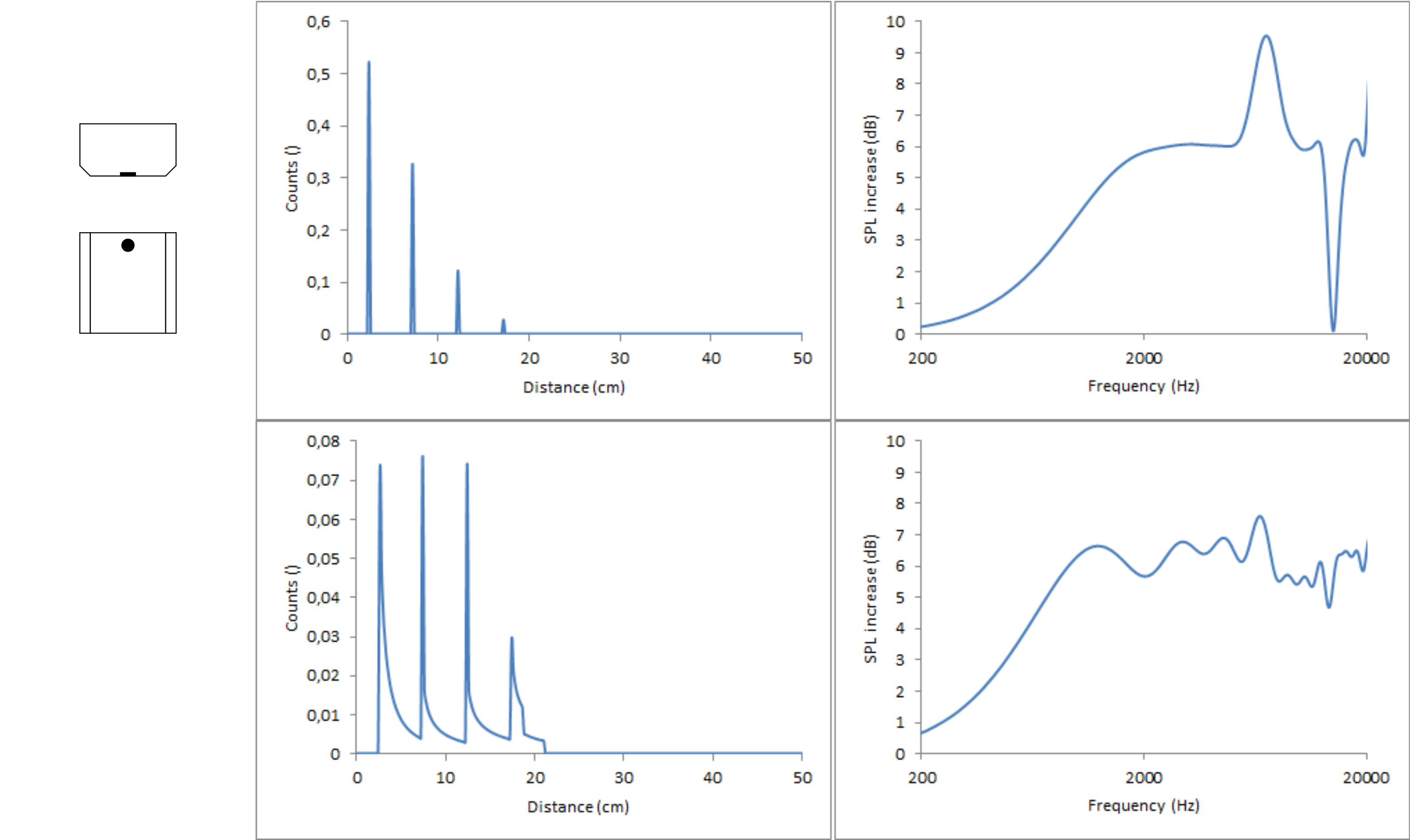
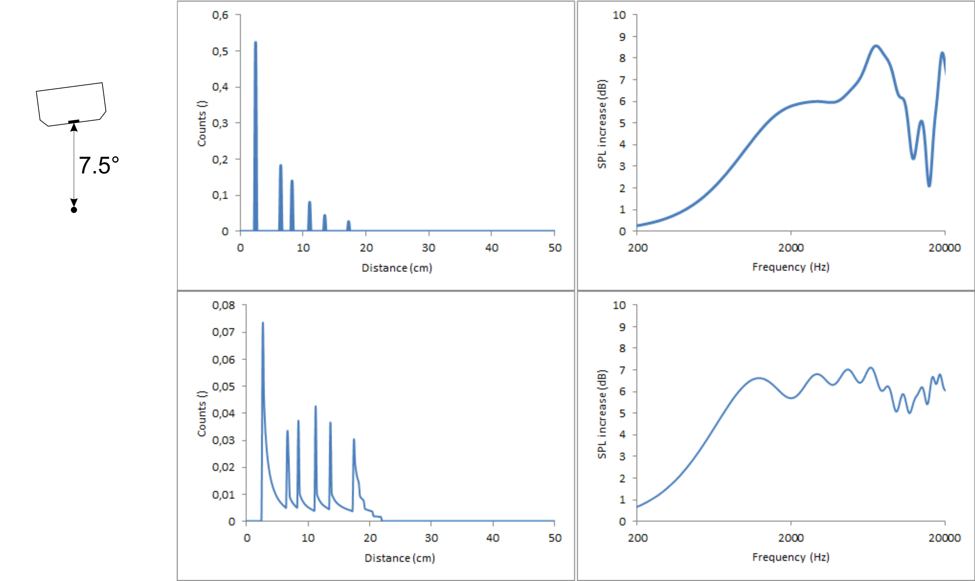
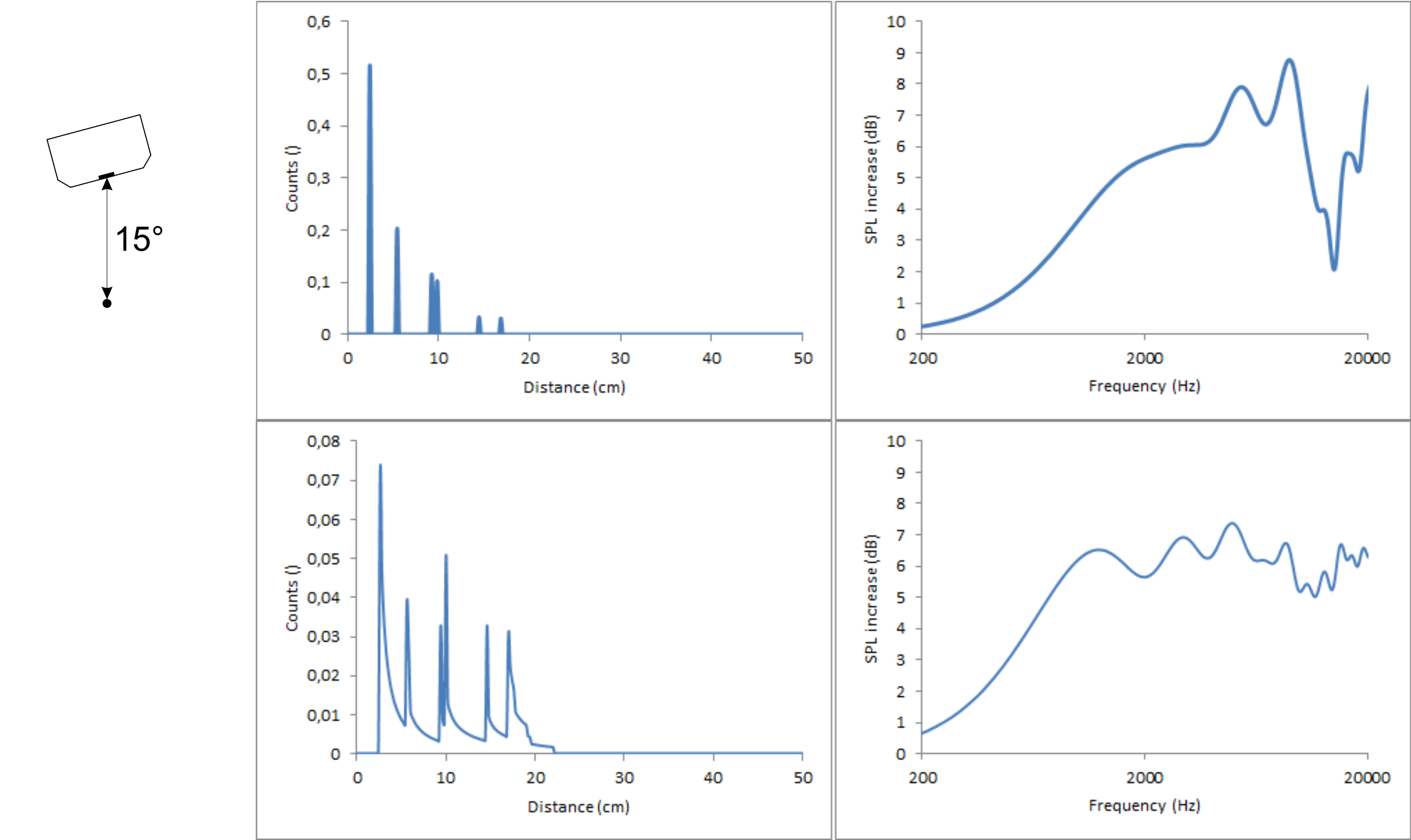
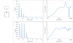
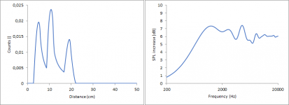
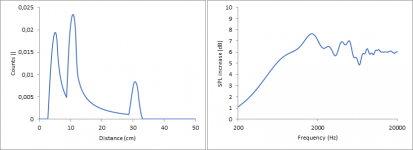
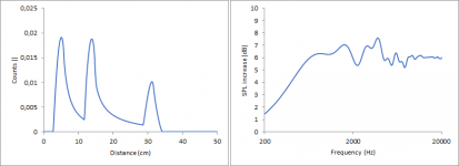
When heavily tilting the speaker it still gives the same behaviour: There are 4 edges, so there will be 4 peaks in the count vs distance graph each starting with a steep step and then decaying going to higher distances. Focusing on the on-axis behaviour of the second image, since the tweeter is placed in the middle of the baffle, the distance to the left and right edge will overlap. Overall there will be a weaker peak at a small distance, a strong peak somewhere in the middle due to the combination of left and right and another weak peak at higher distances, very much like the first picture in post #5. The precise position of the peaks then depends on the dimensions of the baffle.
When heavily tilting the speaker it still gives the same behaviour: There are 4 edges, so there will be 4 peaks in the count vs distance graph each starting with a steep step and then decaying going to higher distances. Focusing on the on-axis behaviour of the second image, since the tweeter is placed in the middle of the baffle, the distance to the left and right edge will overlap. Overall there will be a weaker peak at a small distance, a strong peak somewhere in the middle due to the combination of left and right and another weak peak at higher distances, very much like the first picture in post #5. The precise position of the peaks then depends on the dimensions of the baffle.
Ps. Have You taken into account that the listening axis is not only off but also diagonal vs the loudspeaker axis of symmetry?
I am fairly certain about my qualitative description of the count vs distance graph and therefore about the way how to describe the diffraction pattern for such a baffle.
The resulting diffraction pattern is a different story since it depends heavily on where exactly those peaks in the count vs distance graph are positioned. The diffraction pattern may look like the first picture in post #5 but it may also look like any of the attached pictures.
The exact diffraction pattern can only be determined if the dimensions and angles of the speaker are known.
Attachments
How about some really heavy tilt? Like in case of Shahinian or Heed speakers?
This aria from another "opera".
")
And on the topic: there are theoretical calculations and programs, and there are natural measurements with a microphone and the ability to correctly build the separation filter. And these are the different poles of a large planet.
There are some additional math details in the description of the baffle diffraction algorithm used in the Passive Speaker Designer (PSD) at this URL: PASSIVE SPEAKER DESIGNER
Here is the "manual" for the Baffle Designer in PSD: PASSIVE SPEAKER DESIGNER
When I was working on the code, my primary source of information was Paul Verdone's Operator's Manual for the Baffle Diffraction Simulator. There is a copy of that document here: Operator Manual
Here is the "manual" for the Baffle Designer in PSD: PASSIVE SPEAKER DESIGNER
When I was working on the code, my primary source of information was Paul Verdone's Operator's Manual for the Baffle Diffraction Simulator. There is a copy of that document here: Operator Manual
Ps. Have You taken into account that the listening axis is not only off but also diagonal vs the loudspeaker axis of symmetry?
I was referring to the speakers shown in your second picture and assumed that they are positioned in a way that the front points at the listener. If they are parallel to the wall then you are completly right and it will be different. Then there will be 4 peaks in the count vs distance graph. The same is true for the speakers shown in your first picture.
interesting earlier discussion: What are some good example of baffle design to improve diffraction
- Status
- This old topic is closed. If you want to reopen this topic, contact a moderator using the "Report Post" button.
- Home
- Loudspeakers
- Multi-Way
- How to tame your diffractions