Acoustic Horn Design – The Easy Way (Ath4)

onni · 2019-09-27 7:44 am

mabat said:
I meant that in an axisymmetric situation it is trivially easy to draw anything you wish with just a few lines. And for each line segment you can define a different contribution to the total acoustic output (i.e. its weight) - you should do that for the surround. In a 3D simulation you must allways generete the whole mesh. It's not that hard either, only much more demanding.

BTW, ABEC lets you define the direction of motion for each element - you can easily simulate a vibrating piston/dome or a pulsating spherical cap if you wished. By default the motion is normal to the boundary so for a dome tweeter you will have to change that to the axial direction for all its elements.

Ok, thanks! I'll try this.

/Anton

mabat · 2019-09-27 7:46 am

If you struggled with ABEC I could give you some template or even the simple project generator I have made. It only needs some polishing. Then it's easy to customize.

onni · 2019-09-27 8:37 am

mabat said:
If you struggled with ABEC I could give you some template or even the simple project generator I have made. It only needs some polishing. Then it's easy to customize.

Sure, please do

/Anton

mabat · 2019-09-27 12:46 pm

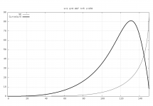
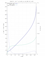
Here is the termination term SE(x) alone (i.e. from OS(x) + SE(x)) with its curvature. It's interesting.

The curvature rises very gently, then for a while it rises almost linearly (i.e. approximates a clothoid), then after reaching the maximum it decreases again. So it is more like two clothoids smootly connected one to another. It makes sense after all, as long as the baffle is flat. It makes a very nice transition from a throat all the way to the baffle.

mabat · 2019-09-27 12:58 pm

n = 3

mabat · 2019-09-27 3:01 pm

Here's the math -

Code:

set term pngcairo size 1000,700 font "Courier New,11"
set output "se_curvature.png"

q = 0.995
s = 0.8
n = 4.5
L = 150

set grid
set size ratio -1
set key top left
set samples 600
set xlabel "x [mm]"
set ylabel "y [mm]"
set xrange [0:L]
set y2range [0:0.05]
set ytics nomirror
set y2tics
set y2label "Curvature"
set title sprintf("s=%g q=%g n=%g L=%g", s, q, n, L)

se(x) = L*s/q * (1.0 - (1.0 - (q*x/L)**n)**(1/n))
fd(x) = L**(1-n) * q**(n-1) * s * x**(n-1) * (1.0 - (q*x/L)**n)**(1/n-1)
sd(x) = (L**(n+1) * (n-1) * q**(n-1) * s * x**(n-2) * (1 - (q*x/L)**n)**(1/n)) / ((q*x)**n - L**n)**2
curv(x) = sd(x) / (1.0 + fd(x)**2)**1.5

plot se(x) axes x1y1 lc rgb "black" t "SE", curv(x) axes x1y2 lw 3 lc rgb "black" t "Curvature"

gedlee · 2019-09-27 4:24 pm

Mabat - it appears to me that you have found the formula for the ideal waveguide. Congratulations. Why everyone is so obsessed with inferior concepts is beyond me.

mabat · 2019-09-27 4:45 pm

Yeah, it seems I've been lucky

Thank you.

Here is the whole thing -

gedlee · 2019-09-27 5:20 pm

NO!! Not lucky. You have exhibited a serious level of hard work - not luck! When Einstein discovered relativity, was it luck? Not at all, it was intuition and hard work, the way virtually all breakthroughs happen.

mabat · 2019-09-27 5:53 pm

I stand on the shoulders of giants

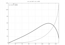
This is all the math involved for those interested to pursue it any further (a gnuplot script producing the above picture):

Code:

# =====================================================================================================
# OSWG-SE gnuplot script; Marcel Batik, 2019
# =====================================================================================================
#
# Input parameters
# -----------------------------------------------------------------------------------------------------
unit = "mm"        # length unit

r = 12.7           # throat radius
tau = 0.0          # throat entry angle [deg]
alpha = 90.0       # coverage angle [deg]
L = 150.0          # lenght(depth) of the waveguide
q = 0.995          # SE parameter
s = 1.0            # SE parameter
n = 5.0            # SE parameter

# -----------------------------------------------------------------------------------------------------
# The maths

set angles degrees

k1 = r*r
k2 = 2.0*r*tan(0.5*tau)
k3 = tan(0.5*alpha)**2.0

# OS profile
os(x) = sqrt(k1 + k2*x + k3*x*x)

# OS first derivative
os1(x) = (k3*x + 0.5*k2) / sqrt(k3*x*x + k2*x + k1)

# OS second derivative
os2(x) = (k1*k3 - 0.25*k2*k2) / (k3*x*x + k2*x + k1)**1.5

# OS curvature
oscurv(x) = os2(x) / (1.0 + os1(x)**2)**1.5

# SE profile
se(x) = L*s/q * (1.0 - (1.0 - (q*x/L)**n)**(1/n))

# SE first derivative
se1(x) = L**(1-n) * q**(n-1) * s * x**(n-1) * (1.0 - (q*x/L)**n)**(1/n-1)

# SE second derivative
se2(x) = (L**(n+1) * (n-1) * q**(n-1) * s * x**(n-2) * (1 - (q*x/L)**n)**(1/n)) / ((q*x)**n - L**n)**2

# SE curvature
securv(x) = se2(x) / (1.0 + se1(x)**2)**1.5

# OS+SE
wg(x) = os(x) + se(x)
wgcurv(x) = (os2(x) + se2(x)) / (1.0 + (os1(x)+se1(x))**2)**1.5

# -----------------------------------------------------------------------------------------------------
# plotting

set term pngcairo size 800,1000 font "Courier New,11"
set output "oswg_se.png"

set grid
set size ratio -1
set key top left
set samples 600
set xlabel sprintf("x [%s]", unit)
set ylabel sprintf("y [%s]", unit)
set xrange [0:L]
set y2range [0:0.1]
set ytics nomirror
set y2tics
set y2label "Curvature"
set title sprintf(\
  "OSWG-SE: r=%g {/Symbol t}=%g {/Symbol a}=%g s=%g q=%g n=%g L=%g", r, tau, alpha, s, q, n, L\
)

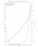
plot os(x) axes x1y1 lc rgb "#a0a0a0" t "OS",\
     se(x) axes x1y1 lc rgb "black" t "SE",\
     securv(x) axes x1y2 lw 3 lc rgb "black" t "SE curv.",\
     wg(x) axes x1y1 lw 1 lc rgb "#7070c0" t "OS+SE",\
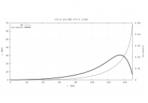
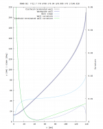
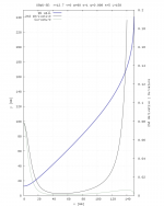
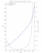
     wgcurv(x) axes x1y2 lc rgb "#7070c0" lw 3 t "OS+SE curv."

mabat · 2019-09-27 8:05 pm

Waveguide wall contour, slope and curvature -

Code:

# =====================================================================================================
# OSWG-SE gnuplot script(2); Marcel Batik, 2019
# =====================================================================================================
#
# Input parameters
# -----------------------------------------------------------------------------------------------------
unit = "mm"        # length unit

r = 12.7           # throat radius
tau = 0.0          # throat entry angle [deg]
alpha = 90.0       # coverage angle [deg]
L = 150.0          # lenght(depth) of the waveguide
q = 0.998          # SE parameter
s = 1.0            # SE parameter
n = 5.0            # SE parameter

# -----------------------------------------------------------------------------------------------------
# The maths

set angles degrees

k1 = r*r
k2 = 2.0*r*tan(0.5*tau)
k3 = tan(0.5*alpha)**2.0

# OS profile
os(x) = sqrt(k1 + k2*x + k3*x*x)

# OS first derivative
os1(x) = (k3*x + 0.5*k2) / sqrt(k3*x*x + k2*x + k1)

# OS second derivative
os2(x) = (k1*k3 - 0.25*k2*k2) / (k3*x*x + k2*x + k1)**1.5

# OS curvature
oscurv(x) = os2(x) / (1.0 + os1(x)**2)**1.5

# SE profile
se(x) = L*s/q * (1.0 - (1.0 - (q*x/L)**n)**(1/n))

# SE first derivative
se1(x) = L**(1-n) * q**(n-1) * s * x**(n-1) * (1.0 - (q*x/L)**n)**(1/n-1)

# SE second derivative
se2(x) = (L**(n+1) * (n-1) * q**(n-1) * s * x**(n-2) * (1 - (q*x/L)**n)**(1/n)) / ((q*x)**n - L**n)**2

# SE curvature
securv(x) = se2(x) / (1.0 + se1(x)**2)**1.5

# OS+SE
wg(x) = os(x) + se(x)
wg1(x) = os1(x) + se1(x)
wgcurv(x) = (os2(x) + se2(x)) / (1.0 + (os1(x)+se1(x))**2)**1.5

# -----------------------------------------------------------------------------------------------------
# plotting

set term pngcairo size 800,1000 font "Courier New,11"
set output "oswg_se.png"

set grid
set size ratio -1
set key top left
set samples 600
set xlabel sprintf("x [%s]", unit)
set ylabel sprintf("y [%s] | slope [deg]", unit)
set xrange [0:L]
set y2range [0:0.1]
set ytics nomirror
set ytics 20
set y2tics
set y2label "Curvature"
set title sprintf(\
  "OSWG-SE: r=%g {/Symbol t}=%g {/Symbol a}=%g s=%g q=%g n=%g L=%g", r, tau, alpha, s, q, n, L\
)

plot wg(x) axes x1y1 lc rgb "#7070c0" lw 3 t "Waveguide wall",\
     atan(wg1(x)) lw 1 t "Wall slope",\
     wgcurv(x) axes x1y2 lw 1 lc rgb "#7070c0" t "Wall curvature"

bmc0 · 2019-09-28 12:36 am

I modified your gnuplot script in order to investigate the difference between a curvature-matched clothoid termination and your new superellipse-based termination.

mabat · 2019-09-28 6:36 am

That's nice. Would be interesting to see how the two wall profiles differ from y=x.

I see this as a minor difference and as you have shown, the acoustic output is almost indistinguishable. What's quite different is the convenience of use. It's really not that easy to work with the clothoids although some claim so

bmc0 · 2019-09-28 8:14 am

I wonder if there could be differences in sound quality that are not obvious in the simulations (higher order modes?). Dr. Geddes has said that the OS contour is optimal because it has the lowest 2nd derivative:

gedlee said:
What one wants to do is to minimize the 2nd derivative - constant would be less than optimal. It can be shown that the OS contour does precisely this, it is a catenoid between the input angle and the output angle. No other function can have a lower 2nd derivative. Now the mouth treatment is another issue and where all the tradeoffs come in.

gedlee said:
Now, of all the surfaces that can connect a circular plane wave to a sperical wavefront, the OS can be proven to genetate the least HOM of any other contour, because it is a catenoid and has a minimum 2nd derivative for a given entry angle.

It seems to me, looking at the graphs, that your new equation has a lower 2nd derivative than the OS+clothoid shape. Perhaps that means that the superellipse-based termination is theoretically superior, even though the simulation results are almost identical (I've done some more sims... the two profiles don't appear to differ by more than a few tenths of a dB out to at least 60°). Thoughts?

mabat · 2019-09-28 9:27 am

I've never really understood this 2nd derivative thing. As a function it will be smoother by itself (I don't know whether "lower" - lower where?), that "feels" better, but to what degree it has any impact, I have no clue.

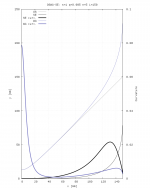
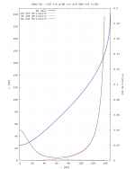
Waveguide with a 2" throat will have lower 2nd derivative near the throat - does it make less HOM because of this?

mabat · 2019-09-28 9:41 am

WG profile, 2nd derivative and curvature, for 1" and 2" throats.

mabat · 2019-09-28 6:13 pm

jzagaja said:
... For compression driver we need different code. I haven't printed it yet because working on printer right now. Author spent whole week on printing these

So do you think it would be possible to place such lens in front of an existing compression driver, shape the wavefront to spherical and use a conical waveguide?
There are several larger format drivers that have a phase plug ending at the very end of the driver, with zero exit angle. That might be an interesting exercise.

gedlee · 2019-09-28 6:36 pm

mabat said:
WG profile, 2nd derivative and curvature, for 1" and 2" throats.

Since the equation for an OS profile only contains the throat radius as a constant, how can the second derivative be different?

mabat · 2019-09-28 6:43 pm

The scale of the hyperbola is different. The larger the throat radius, the smaller the curvature at the throat.

gedlee · 2019-09-28 6:46 pm

Mabat - for an OS waveguide alone that is not possible (look at the equation). Only the term that you added could do that, in which case it is modifying the OS curvature way down at the throat where it is most critical.

Acoustic Horn Design – The Easy Way (Ath4)

Member

Member

Member

Member

Attachments

Member

Attachments

Member

Attachments

Member

Member

Attachments

Member

Member

Member

Attachments

Member

Attachments

Member

Member

Member

Attachments

Member

Attachments

Member

Member

Member

Member