It's unnecessary to consider cantilever flex and inertia separately, rather a transmission line vibration model wraps it all up very elegantly IME. Otherwise, one ends up combining two imperfect models and it's all a bit of a fudge and defies physical explanation, which is unsatisfying I find.
Excellent - I am interested in your model. Perhaps you could start another thread for it?
I've never understood why this analogy is deemed useful, ie why mechanics is not deemed perfectly understandable on its own merit and terms, and yet electrical systems somehow are !?!
Dynamical analogies are (were?) the lingua franca of the engineering world. They helped us exchange ideas and stopped us from re-inventing each other's analyses. They remain very useful in electro-mechanical systems (to name but one field). Richard Small's papers on loudspeakers are an excellent example (one of many).
Well no, the published plot is mechanical impedance to motion of the stylus. Well, strictly the magnitude of mechanical impedance at a specific frequency. It was derived from measured VTF required at the onset of mistracking of a given velocity. It's not great physics, but is OK and it's what was done in the day.
Thanks - if you can point me to it, I would like to read the source. You see, the units on the Y-axis (dyne.sec/cm) are those specified for damping. The annotation is usually quite different for mechanical impedence, which is usually expressed in mechanical ohms to avoid confusion.
Incidentally, impedance at 100Hz was read off, expressed as if it was pure spring, and this is the meaning of compliance at 100Hz as used by Japanese cartridge manufacturers.
I'm afraid not - they are the spring constants at 100Hz, the inverse of the compliance. They are not impedences (there is no ambiguity there).
Excellent - I am interested in your model. Perhaps you could start another thread for it?
Why does it need another thread? Seems entirely on topic for this thread. The equations were posted early on in the thread.
Thesis is that mechanical resonance, the topic of this thread, can be explained by propagation of transverse vibrations along the cantilever, and can be modelled as a mechanical transmission line. As such, I think discussion is best left on this thread for now, since I think the crux of this thread closely involves it.Excellent - I am interested in your model. Perhaps you could start another thread for it?
Analogies are common enough, but it's better to deal with mechanical analysis in proper terms on its own merit, I think. An example might be that mechanical transmission lines here are typically quite dispersive, whereas electrical ones generally aren't (very)......Dynamical analogies are (were?) the lingua franca of the engineering world. They helped us exchange ideas and stopped us from re-inventing each other's analyses. They remain very useful in electro-mechanical systems (to name but one field). Richard Small's papers on loudspeakers are an excellent example (one of many).
Damping and mechanical impedance have the same dimensions, force per velocity. Damping is always entirely real, whereas impedance isn't necessarily so. For sure, that is a plot of magnitude of mechanical impedance. At any single frequency, spring and inertia express an impedance which is complex, but has a magnitude, of course. Damping expresses an impedance which is always real.Thanks - if you can point me to it, I would like to read the source. You see, the units on the Y-axis (dyne.sec/cm) are those specified for damping. The annotation is usually quite different for mechanical impedence, which is usually expressed in mechanical ohms to avoid confusion.
The plot, IIRC, is from a Yamamoto book published by JVC. Reference for which is on Yosh's excellent recspec site, including a brief narrative of the derivation and meaning of the mechanical impedance plots.
It is mechanical impedance at 100Hz, read from the plot, and expressed as if it came from a pure spring. Which is not quite physically the same as the spring constant at 100Hz, because in practice at 100Hz, most of the impedance comes from damping not the suspension spring. This is why the 'spring constant' or 'compliance' as published is so different between 10Hz and 100Hz. As posted, not my idea of good physics, but it is what was done back in the day.I'm afraid not - they are the spring constants at 100Hz, the inverse of the compliance. They are not impedences (there is no ambiguity there).
LD
Why does it need another thread? Seems entirely on topic for this thread. The equations were posted early on in the thread.
Thanks, billshurv - found summary mechanical parameters at post 82 and the transmission line model at post 60 - thank you luckythedog.
Lucky, I see that the cantilever mechanism is modelled as a transmission line, Length = 2000 (I assume metres?), L = 250nH/m and C = 100pF/m. The transmission line is parallel with an AC voltage source and a 10 Ohm resistance. Can you please walk us through the transformation of the mechanical parameters that you derived into the electrical analogs that you modelled?
PS: Do you have the reference for the Happ/Shibata paper you referred to in post #60? Ta.
PPS: Found a number of Yamamoto's charts on Yoshi's site, but not the chart we were discussing. Do you have a link? Ta.
Last edited:
That transmission line model sketch is an illustration, another spherical cow (!), but shows the principle at issue nicely I think.Lucky, I see that the cantilever mechanism is modelled as a transmission line, Length = 2000 (I assume metres?), L = 250nH/m and C = 100pF/m. The transmission line is parallel with an AC voltage source and a 10 Ohm resistance. Can you please walk us through the transformation of the mechanical parameters that you derived into the electrical analogs that you modelled?
In defence of using an electrical model, both mechanical and electrical systems are in play, and so, to simulate the whole thing one needs to chose, and spice is pretty convenient. However, the mechanical TL in this case should be dispersive, ie tprop should depend on f, but the TL spice model I used doesn't support that, neither did I insert any loss.
TL length is chosen to mimic realistic physical transverse wave propagation along the cantilever: mechanical transverse waves are slow, and certainly so compared to electronic lines. So a line length of 2000 metres or so gives about the right tprop. NB, at issue is not the speed of sound in the cantilever, which are compression waves, rather it is velocity of a transverse wave.
Line impedance, set by L and C, is chosen to provide a normal workable impedance and tprop for the line, 50R IIRC. Source and termination impedances are chosen to suitably mismatch the line impedance, representing overterminated source and underterminated load, ie driven stylus and free (but complex) generator.
What it shows, I think, is that both the form of solution, ie the transfer function of the whole cartridge, and specific response can reasonably realistically mimic reality, from a relatively simple TL cantilever model.
Found a number of Yamamoto's charts on Yoshi's site, but not the chart we were discussing. Do you have a link?
ƒeƒXƒgƒŒƒR�[ƒh
The whole page is worth a read, and parts are in Japanese.
Also referenced is a Denon test record XG-7001 with instructions for how to calculate and plot and a mechanical impedance curve for a cartridge, by observing limit of trackability.
That might take a short time. Everything is somewhere !PS: Do you have the reference for the Happ/Shibata paper you referred to in post #60?
LD
Last edited:
AT have discontinued the AT400MLb so was having a look at the replacement. Its 20% more expensive but does now use a tapered thinwall cantilever. They seem to have standardised over that in all of the better models and the differentiation is now the stylus. Interestingly the previously top of the line microline is now #3 , shibata #2 and 'special line contact' at #1. Go figure! I need to start another thread on the twists and turns of stylus of the day. 'special line contact' is £500 for a replacement stylus. erm no thanks.
Reason for the ramble is, how does a taper change the transmission line properties? It affects resonant frequency (usually broadening the Q), but in a world where the transmission line model holds how does one model it (and does it matter)?
Reason for the ramble is, how does a taper change the transmission line properties? It affects resonant frequency (usually broadening the Q), but in a world where the transmission line model holds how does one model it (and does it matter)?
Referring to the Aurak Virtual input preamp that was discussed and simulated earlier in this thread, LTSpice measured the balanced version having 3 dB less S/N ref 5mV @ 1Khz as opposed to the SE version.
It took me a while to understand why, but the solution is of course quite simple.
When using virtual inputs, both sides of the balanced inputs do receive the same current in opposite direction causing the sum of both halves to producing twice the output voltage of an SE version with only 3dB more noise.
Ergo, S/N has increased with 3dB for a Virtual Input Balanced Aurak.
By interchanging the 4k2 and 5k4 resistors around the input OPA, Freq Response and Gain stay exactly the same but noise is reduced by another 1dB, easy to explain, but left out here.
Overall gain for the balanced version will be 49dB with components as shown in #206, so gain of the second part doing the 3180 us and 318 us correction could be made a bit lower.
So to conclude: A balanced version of the Aurak as in posting #206, but with the 4.2K and 5.4K resistors interchanged has a 4dB better S/N ref 5mV@1Khz (72.8 dB using the OPA1642) compared to the SE version as in posting #204.
A balanced voltage amplifier however does not offer twice the gain but exactly the same gain as an SE version, but noise penalty is here also 3 dB.
So S/N decreases by 3dB when using a balanced voltage amplifier.
Hans
OK - I can see where you're coming from
There are wrinkles I see from the mechanical perspective, but none of them need be a “killer”.
Can we take a cart with a known Effective Tip Mass and feed its dimensions into the transmission line model to generate an estimate of the first mechanical resonance? Then, plugging the Effective Tip Mass and modelled Fres into a single degree of freedom lumped mass model, does it give an estimate of compliance close to but not too much bigger than L^3/3EI? If so, you may have a winner!
PS: Thanks for the link to the mechanical impedence curves - I think that Denon's documentation for its test disc is what is needed, or the help of a Japanese translator, or both.
Still here
I left the mixed analog digital EQ as a future study in my article and would gladly look at some kind of cookbook for non-traditional RIAA. Some of the circuits that have passed by get to be a mess of op-amps and time constants better done in digital with today's capabilities.
I left the mixed analog digital EQ as a future study in my article and would gladly look at some kind of cookbook for non-traditional RIAA. Some of the circuits that have passed by get to be a mess of op-amps and time constants better done in digital with today's capabilities.
OOOPS! should have been TOTAL mass
My apologies, Lucky. In my eagerness to reconcile your model with the classic model, I made a mistake. It's the total mass of the cantilever (not the effective tip mass) that needs to be used.
Then, plugging the Effective Tip Mass and modelled Fres into a single degree of freedom lumped mass model
My apologies, Lucky. In my eagerness to reconcile your model with the classic model, I made a mistake. It's the total mass of the cantilever (not the effective tip mass) that needs to be used.
Scott: don't rush on my behalf as not only 2 years behind on projects* but still not worked out which way to jump. Luckily the (minimal) pre-sets on miniDSP mean I can have the 3 likely options (Flat, LF only, full RIAA) programmed in.
Madness of course would occur if I stuck a behringer DEQ2496 in the way. I thought about the whole 'performance controls' bit and decided that's offline processing.
*last time I took a week off to catch up on projects both cars decided to break down on the same day!
Madness of course would occur if I stuck a behringer DEQ2496 in the way. I thought about the whole 'performance controls' bit and decided that's offline processing.
*last time I took a week off to catch up on projects both cars decided to break down on the same day!
and would gladly look at some kind of cookbook for non-traditional RIAA. Some of the circuits that have passed by get to be a mess of op-amps and time constants better done in digital with today's capabilities.
I guess the JLH Liniac version in John Broskie’s tubecad #373 is one of the non-traditional RIAA arrangements, although simple and with standard component values (*)
In simulation it behaves very well.
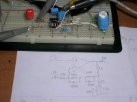
I bread boarded it today with a TL082 in place of the liniac amp, intentionally a bit of a mess to check if it oscillates, amazingly though it doesn’t.

I’ll build a proper dead bug version on copper sheet and I’ll report back
(*) the original article
http://www.keith-snook.info/wireless-world-magazine/Wireless-World-1971/The%20Liniac%20by%20John%20L%20Linsley%20Hood.pdf
George
Attachments
I guess the JLH Liniac version in John Broskie’s tubecad #373 is one of the non-traditional RIAA arrangements, although simple and with standard component values (*)
In simulation it behaves very well.
I bread boarded it today with a TL082 in place of the liniac amp, intentionally a bit of a mess to check if it oscillates, amazingly though it doesn’t.
I’ll build a proper dead bug version on copper sheet and I’ll report back
(*) the original article
http://www.keith-snook.info/wireless-world-magazine/Wireless-World-1971/The%20Liniac%20by%20John%20L%20Linsley%20Hood.pdf
George
Capacitor soakage, much ado about nothing.
Scott: don't rush on my behalf
No hurries, ran across another one today Direct-Disk Labs Guitar Wizard, Thumbs Carlille playing covers of "Just the way you are" and "Stayin' Alive" , etc. on one of the most open natural and fine LP's I have heard. Frustrating.
EDIT - Went for the antidote, Segovia's 1959 recording of Concierto del Sur and as Decca asked I used RIAA for proper stereo reproduction. I should spend a day doing the hand removal of ticks from this amazing recording.
Last edited:
I thought you have automatic declicking? I will have to look this one up.
Me, automatic anything? BTW DL710027
Last edited:
Well pretty sure your wife's car isn't available with stick shift
You do often recommend a click repair package so assumed you sometimes used it?
None that work while you play, offline only. Sad as it may seem I just put on the LP's and listen most of the time.
I wonder what Audi would do if you wanted a Q7 with manual, these days no amount of money would convince them. The wife is gone this week and I get to drive it and maybe figure out all the systems, hopeless.
Last edited:
- Home
- Source & Line
- Analogue Source
- mechanical resonance in MMs