cap'n todd said:
Hi John, so are you trying to remove all ringing then? Then add some back in to make it sound more natural? I'm dont really think its necessary, but sounds interesting.
I actually think this is a done deal. I have to modify my simulation code before I can verify it theoretically though. And right now I really don't feel like writing code.
")
youngho, no, I was talking about the rate after the initial drop. Looking at the picture Todd posted, the line on the left hand side decays faster than that on the right side. In the first few ms there's a huge drop but we still do not know if this is enough to render the ringing inaudible.
Todd offers an explanation:
But doesn't this bring us back to my initial comment that I've never seen a CSD that clearly shows that an EQ completely eliminated ringing?
Todd offers an explanation:
So you end up with a corrected response that has two slopes, from the Q of the resonance and the correction filter not cancelling correctly. Should it be surprising that the decay in time has two slopes then?
But doesn't this bring us back to my initial comment that I've never seen a CSD that clearly shows that an EQ completely eliminated ringing?
markus76 said:youngho, no, I was talking about the rate after the initial drop. Looking at the picture Todd posted, the line on the left hand side decays faster than that on the right side. In the first few ms there's a huge drop but we still do not know if this is enough to render the ringing inaudible.
Hmm, it goes to zero on the right earlier, no? It decays faster on the right initially, then it seems to decay more slowly after that, but it reaches zero earlier. And shouldn't inaudible should be at the level of the noise floor?
Oops, sorry, not a physicist or an engineer. I'l shut up now.
youngho said:And shouldn't inaudible should be at the level of the noise floor?
It should be inaudible if the noise floor is inaudible
I think the data shown isn't very clear, but it was not me that asserted that "This [data] is not hard to find." markus76 said:
It should be inaudible if the noise floor is inaudible
Just out of curiosity, how would this "modal ringing" be audible above the noise floor, i.e. the "room ringing"? And the graphs were in the book! I was about to refer you to page two-hundred-forty-whatever, myself.
john k... said:
Earl you missinterpreted what I posted, due to my poor gramar.
How about if I rewrote that as, "In simple terms, X must satisfy the wave equation with no sources in the interior. Boundary conditions as required are applied so that when added to g, g + X = G, the solution for the bounded region."
I would agree that solving the wave equation, with appropriate boundary conditions, for X might not be an easy task, but someone must have done it to come up with the modal expansion for G. So, X = G-g must at least be a reasonable representation of X, at least as good as G is a representation of the bounded region Green's function.
John
Agreed! With one caveat. The function X(r) will be different for every source position in the room. There is no single X(r) that will satisfy the boundary conditions for an arbitray source location.
When Morse subtracts off the near field from the Green's function G(r) he does this by only fitting the singularity at the source point. This approach is then only approximate at the walls, but more accurate at the source than the series, because it converges faster. This leaves X(r) independent of the source location, BUT it is only an approximate solution.
markus76 said:
It should be inaudible if the noise floor is inaudible
I could definately find more, but it is time consuming. If yo have access to the AES journal, you should find more. And in any case I agree that the waterfalls are often hard to read/interpret.
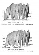
Here's one I measured myself, a resonance at 28 Hz, no eq and eq.
Attachments
gedlee said:
John
Agreed! With one caveat. The function X(r) will be different for every source position in the room. There is no single X(r) that will satisfy the boundary conditions for an arbitrary source location.
When Morse subtracts off the near field from the Green's function G(r) he does this by only fitting the singularity at the source point. This approach is then only approximate at the walls, but more accurate at the source than the series, because it converges faster. This leaves X(r) independent of the source location, BUT it is only an approximate solution.
I think the problem is the way Morse write the relationship
G(R,Ro) = g(R,Ro) + X(R)
This says X(R) = G(R,Ro) -g(R,Ro) .
Obviously X is a function of Ro. However, X(R) is a solution to (here we go again) the homogeneous wave equation with inhomogeneous boundary conditions (finally got that right). This is were the dependents of X(R) on Ro comes in because the boundary conditions are dependent upon the value of g(R,Ro) evaluated on the bounding surfaces. So while the dependence of X on Ro is not explicit, there is implicit dependence of X on Ro from the BC's. Perhaps it would have been better if Morse had written X(R) is a solution to the homogeneous wave equation with inhomogeneous boundary conditions, BC = F(g(Rb,Ro)) where Rb is the position vector defining the bounding surface. Change the source position and the X changes as well.
I guess I saying that I'm not particularly worried about what Morse says he does or doesn't do. If I have G(R,Ro) and I know g(R,Ro) I can drop in the values of R and Ro and find the value of X (R) for any values of R and Ro in the bounded region. But it's all academic because there is no need to worry about X if we know G(R,Ro).
On the effect of EQ on decay rate
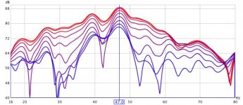
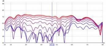
By courtesy of the Anti-Mode 8033 subwoofer EQ developer I'm posting a before/after comparison of what the aforementioned little box can do with regards to the decay rate of LF modes.
The time slices are 20 ms each, so from 0-160 ms. The comparison clearly shows faster rate of decay, at least up to 160 ms.
Attachments
markus76 said:Looks like this box is pretty effective if you want to automatically EQ a single listening position. 225 Euros is ok.
Best, Markus
I think that was Todds point earlier. If all you want to do is a single point then its a far easiler problem.
john k... said:
I think the problem is the way Morse write the relationship
G(R,Ro) = g(R,Ro) + X(R)
This says X(R) = G(R,Ro) -g(R,Ro) .
Obviously X is a function of Ro. However, X(R) is a solution to (here we go again) the homogeneous wave equation with inhomogeneous boundary conditions (finally got that right). This is were the dependents of X(R) on Ro comes in because the boundary conditions are dependent upon the value of g(R,Ro) evaluated on the bounding surfaces. So while the dependence of X on Ro is not explicit, there is implicit dependence of X on Ro from the BC's. Perhaps it would have been better if Morse had written X(R) is a solution to the homogeneous wave equation with inhomogeneous boundary conditions, BC = F(g(Rb,Ro)) where Rb is the position vector defining the bounding surface. Change the source position and the X changes as well.
I guess I saying that I'm not particularly worried about what Morse says he does or doesn't do. If I have G(R,Ro) and I know g(R,Ro) I can drop in the values of R and Ro and find the value of X (R) for any values of R and Ro in the bounded region. But it's all academic because there is no need to worry about X if we know G(R,Ro).
John
Agreed. I had always viewed this subtraction of the direct field as approximate at the boundaries, never exact. I think that's the part that may be getting lost. You are correct that G(r,r0) is exact and what is needed, it just converges very slow near the source. I suppose that one could use the near field term for points close to the source, but drop it further out. This would work if the source is not too close to a boundary. If the source is close to a boundary then using an image source or sources would work as the combination is always zero at the boundary.
gedlee said:I think that was Todds point earlier. If all you want to do is a single point then its a far easiler problem.
I didn't argue against using an EQ. I just expressed my doubts that ringing can be completely eliminated in a real room by applying an EQ.
Talking about that box, how does it determine the target magnitude?
Best, Markus
markus76 said:
I was about to laugh, then I saw that it is "Room Perfect", which was developed by Jan Pedersen, for Lyngdorf. At least there's some science involved.
- Home
- Loudspeakers
- Subwoofers
- Multiple Small Subs - Geddes Approach