It seems there is another bug in the Compound Horn feature.
Hi witasso,
Many thanks for the feedback - for a change, this one is not a bug
") .
.By way of explanation - for the given example, two equal outputs 180 degrees out of phase and with a zero path length difference are being combined. The two radiated signals effectively cancel each other out which is why the calculated value of the combined SPL response is effectively non-existent at less than -200 dB.
Any change in dimensions, no matter how small, will have a significant effect on the results.
Kind regards,
David
Bug Fixed
Hi David_Web,
The bug you identified has now been fixed. The latest Hornresp release is Product Number 2800-100826. Thanks again for the feedback.
Kind regards,
David
Getting some strange result in the loudspeaker wizard with this one using combined response.
Hi David_Web,
The bug you identified has now been fixed. The latest Hornresp release is Product Number 2800-100826. Thanks again for the feedback.
Kind regards,
David
Hi David,
Thanks for the continuing effort, just down-loaded 2800-100826, and have not found any bug yet.
Would it be possible to add the Compound Horn to the Loudspeaker Wizard with the "Response-Default-Output 2-Combined" feature as it is available for the bass reflex speaker?
Regards,
Thanks for the continuing effort, just down-loaded 2800-100826, and have not found any bug yet.
Would it be possible to add the Compound Horn to the Loudspeaker Wizard with the "Response-Default-Output 2-Combined" feature as it is available for the bass reflex speaker?
Regards,
Hi Oliver,
Excellent news, but please keep searching.
That's interesting, I thought the feature was already there. It works fine for me.
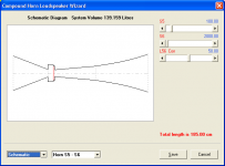
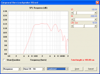
Note the "Compound Horn Loudspeaker Wizard" heading and the "Horn S5 - S6" and "Combined" options selected on the attached example screenprints. Can't you get the same thing, using the following data?
ID=28.00
Ang=0.5 x Pi
Eg=2.83
Rg=0.00
Cir=1.00
S1=80.00
S2=350.00
Con=60.00
F12=0.00
S2=350.00
S3=2400.00
Exp=75.00
F23=70.27
S3=0.00
S4=0.00
L34=0.00
F34=0.00
S5=100.00
S6=2000.00
Con=50.00
F56=0.00
Sd=350.00
Bl=18.00
Cms=4.00E-04
Rms=4.00
Mmd=20.00
Le=1.00
Re=6.00
CH=1
Vrc=4.00
Lrc=8.00
Ap1=0.00
Lpt=0.00
Vtc=900.00
Atc=350.00
Pmax=200
Xmax=5.0
Comment=Compound horn
Kind regards,
David
Thanks for the continuing effort, just down-loaded 2800-100826, and have not found any bug yet.
Excellent news, but please keep searching
.Would it be possible to add the Compound Horn to the Loudspeaker Wizard with the "Response-Default-Output 2-Combined" feature as it is available for the bass reflex speaker?
That's interesting, I thought the feature was already there. It works fine for me
.Note the "Compound Horn Loudspeaker Wizard" heading and the "Horn S5 - S6" and "Combined" options selected on the attached example screenprints. Can't you get the same thing, using the following data?
ID=28.00
Ang=0.5 x Pi
Eg=2.83
Rg=0.00
Cir=1.00
S1=80.00
S2=350.00
Con=60.00
F12=0.00
S2=350.00
S3=2400.00
Exp=75.00
F23=70.27
S3=0.00
S4=0.00
L34=0.00
F34=0.00
S5=100.00
S6=2000.00
Con=50.00
F56=0.00
Sd=350.00
Bl=18.00
Cms=4.00E-04
Rms=4.00
Mmd=20.00
Le=1.00
Re=6.00
CH=1
Vrc=4.00
Lrc=8.00
Ap1=0.00
Lpt=0.00
Vtc=900.00
Atc=350.00
Pmax=200
Xmax=5.0
Comment=Compound horn
Kind regards,
David
Attachments
Compound Horn - Wizard
Hi David,
Thank you for the quick response. As you said it works, the difference is that I didn't break down the front horn into two sections (didn't use S2/S3/L23.) When I added values there the Wizard appeared, and worked great.
Original, no Wizard:
ID=28.00
Ang=2.0 x Pi
Eg=2.83
Rg=0.00
Cir=3.80
S1=400.00
S2=6000.00
Exp=22.00
F12=336.96
S2=0.00
S3=0.00
L23=0.00
AT=34.78
S3=0.00
S4=0.00
L34=0.00
F34=0.00
S5=300.00
S6=301.00
Con=40.00
F56=0.00
Sd=814.00
Bl=20.13
Cms=1.60E-04
Rms=1.98
Mmd=108.79
Le=2.02
Re=6.60
CH=1
Vrc=162.00
Lrc=40.00
Ap1=400.00
Lpt=1.80
Vtc=1600.00
Atc=900.00
Pmax=100
Xmax=5.0
Comment=Compound_Selenium_WPU1507_Le @ Fs_compound_short_example
New, Wizard works:
ID=28.00
Ang=2.0 x Pi
Eg=2.83
Rg=0.00
Cir=4.14
S1=400.00
S2=400.10
Con=1.80
F12=0.00
S2=400.10
S3=6000.00
Exp=20.20
F23=366.96
S3=0.00
S4=0.00
L34=0.00
F34=0.00
S5=300.00
S6=301.00
Con=40.00
F56=0.00
Sd=814.00
Bl=20.13
Cms=1.60E-04
Rms=1.98
Mmd=108.79
Le=2.02
Re=6.60
CH=1
Vrc=162.00
Lrc=40.00
Ap1=0.00
Lpt=0.00
Vtc=1600.00
Atc=900.00
Pmax=100
Xmax=5.0
Comment=Compound_Selenium_WPU1507_Le @ Fs_compound_short_example
Thanks again,
Regards,
Last edited:
As you said it works, the difference is that I didn't break down the front horn into two sections (didn't use S2/S3/L23.)
Hi Oliver,
As indicated in the Hornresp Help file, the Loudspeaker Wizard works with single segment conical and parabolic horns, and all multiple segment horns. In your original design you had a single segment exponential horn. It is necessary to place these restrictions on the Loudspeaker Wizard so that the plane wavefront model is used in all cases - calculation times associated with the isophase model are too slow for it to be applied to the Wizard.
If you have a single segment exponential horn with parameter values S1, S2 and L12, then probably the easiest way to convert it into two segments for the purposes of using the Wizard, is as follows:
Segment 1:
Throat = S1
Mouth = S2
Length (Exp) = L12 - 0.01
Segment 2:
Throat = S2
Mouth = S2
Length (Exp) = 0.01
The very short cylinder at the horn mouth will make no perceptible difference to the overall results.
Kind regards,
David
Last edited:
Hello Michael,
Thanks for the kind words about the spectrogram feature in Hornresp.
What you surely noticed is it's speed and it's smoothness while keeping fine resolution). It takes a few seconds to run (after the IR response has been previously calculated). And remember Hornresp uses VBA as computing language, the speed of which one is quite slow.
(Eventually, if David is OK for that I can reveal a few tricks of my own about how to perform high speed quasi gaussian windowing and the fast sliding Fourier transform-not FFT.)
If I take your 2 reference frequencies 300Hz and 100Hz: the 300Hz shows on the spectrogram a red brick color (around 0dB ) and the 100Hz shows a yellow color (around -15dB). See attached graph. That's the difference of SPL between 30Hz and 100Hz we can see on the Power response curve.
But when analyzing a spectrogram we must also consider that the low frequency part of the IR spreads on a much more larger duration that the high frequency part. For a given frequency one point of the response curve has to be considered as the summation of the magnitude corresponding to the level of the spectrogram along the time width of the spectrogram. A smaller level on the spectrogram for a given low frequency component than for a high frequency component may results, due to its longer duration, in a larger level on the response curve (SPL curve).
Finally, the shape of the "convolving element" used to obtain the spectrogram while chosen in order to reduce at minimum wings effects (as we used to discuss about the choice of parameters for the CSD in ARTA) has a smoothing effect both in frequency and in time on the spectrogram, so, due to the finite(frequency / time) limits of the spectrogram window chosen we may have some smoothing effect on the border of the spectrogram (and specially around the 40Hz border).
Best regards from Paris, France
Jean-Michel Le Cléac'h
David, Jean-Michel - this spectrogram feature is smashing !!
Thanks for the kind words about the spectrogram feature in Hornresp.
What you surely noticed is it's speed and it's smoothness while keeping fine resolution). It takes a few seconds to run (after the IR response has been previously calculated). And remember Hornresp uses VBA as computing language, the speed of which one is quite slow.
(Eventually, if David is OK for that I can reveal a few tricks of my own about how to perform high speed quasi gaussian windowing and the fast sliding Fourier transform-not FFT.)
One thing I noticed is that the spectrogram seems to have different SPL scaling than the SPL plot.
Comparing the difference in SPL from 300Hz and 100Hz its about 30-40dB indicated by the spectrogram whereas its at a more realistic 15dB in the SPL plot ?
If I take your 2 reference frequencies 300Hz and 100Hz: the 300Hz shows on the spectrogram a red brick color (around 0dB ) and the 100Hz shows a yellow color (around -15dB). See attached graph. That's the difference of SPL between 30Hz and 100Hz we can see on the Power response curve.
But when analyzing a spectrogram we must also consider that the low frequency part of the IR spreads on a much more larger duration that the high frequency part. For a given frequency one point of the response curve has to be considered as the summation of the magnitude corresponding to the level of the spectrogram along the time width of the spectrogram. A smaller level on the spectrogram for a given low frequency component than for a high frequency component may results, due to its longer duration, in a larger level on the response curve (SPL curve).
Finally, the shape of the "convolving element" used to obtain the spectrogram while chosen in order to reduce at minimum wings effects (as we used to discuss about the choice of parameters for the CSD in ARTA) has a smoothing effect both in frequency and in time on the spectrogram, so, due to the finite(frequency / time) limits of the spectrogram window chosen we may have some smoothing effect on the border of the spectrogram (and specially around the 40Hz border).
Best regards from Paris, France
Jean-Michel Le Cléac'h
Attachments
Last edited:
(Eventually, if David is OK for that I can reveal a few tricks of my own about how to perform high speed quasi gaussian windowing and the fast sliding Fourier transform-not FFT.)
Jean-Michel Le Cléac'h
Yes sure, I would be very much interested in this !
As for the rest - I must have been "slightly off" to not see it correctly - thanks for putting it right.
Michael
Eventually, if David is OK for that I can reveal a few tricks of my own about how to perform high speed quasi gaussian windowing and the fast sliding Fourier transform-not FFT.
Hi Jean-Michel,
Not a problem
.Welcome back.
Kind regards,
David
I thought I read somewhere that there was a way to get a JMLC round horn. Am I right? How?
Hi pumpkin1,
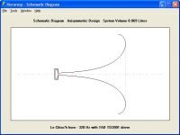
Axisymmetric Le Cléac’h horns can be simulated in Hornresp by selecting the Lec flare option. Horn dimensions can be exported from the Schematic Diagram Window. See the Help file for details.
Kind regards,
David
Attachments
I'm using a Radian 850pb in a 300hz round horn. How important is knowing the exit angle of 10% as well as the length of the base of the horn?
Hi pumpkin1,
I am not sure that I understand exactly what you mean by "exit angle of 10%" and "length of the base of the horn".
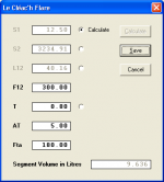
If however (for example) you wish to design a full-mouth 300Hz T = 0.80 Le Cléac’h horn having a throat entry half-angle of 5 degrees (10 degrees included angle) to match a given compression driver exit angle, then this can be readily done using the Horn Segment Wizard. The horn axial length in this case will be 40.16 cm. See attached screenprint.
Kind regards.
David
Attachments
Hi Pumpkin1,
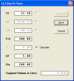
Further to my previous message, the Horn Segment Wizard can also be used to design a Le Cléac’h horn given parameters S1, F12, AT and Fta, rather than F12, T, AT and Fta, if so desired.
This allows the compression driver to be connected directly to the horn throat, without the need for a conical transition piece to match the compression driver exit diameter to that of the horn throat.
Kind regards,
David
Attachments
Last edited:
Yes sure, I would be very much interested in this !
Hello Michael,
First we have to remember that when it comes to operations on arrays or when it comes to symbolic calculation (e.g. as with complex numbers expressed as exp[ait] ) Visual Basic is not that efficient. Even calculations using thousands of cos, sin, exp, etc. are very slow. Better to limit their number.
The spectrogram used in Hornresp on the Impulse Response is of the quasi wavelets type we have yet discussed on DiyAudio. That means that is operates with a sliding Fourier transform. But there is 4 original things:
1) the width of the Fourier window varies as the inverse of the frequency;
2) FFT is not used;
3) the Fourier window has a bell shape
4) convolution product is replaced by a simpler calculation.
The problem with FFT is that it uses discrete frequencies linearly set between 0Hz and Fs. This means that there is the same number of calculated values between the important interval 0 and 1000Hz and the interval 19000 and 20000Hz. As our audition is sensible to the log of the frequency in fact we don’t need the same increment between 2 frequencies at HF than at LF.
If you have ever used Adobe Audition (previously CoolEdit) you’ll see that as its spectrogram is based on FFT and it uses a linear frequency scale. This is a real pity and such spectrogram is nearly useless.
The spectrogram in Hornresp uses a log frequency scale and this allows that fewer values are calculated. From this results a first reduction of the run time.
A classic type of quasiwavelets spectrogram use at each frequency a convolution between the Impulse Response and a convolving pulse, the envelop of which (Fourier window) is a raised cosine or more rarely a Gauss curve. Those as 2 bell shape curves. The calculation of such convolving pulse and then the convolution leads to very long run times, incompatible with the use of Hornresp.
The problem is very much easier when the shape of the Fourier window is rectangular. It allows the use of Sliding Fourier Transform (SFT) much easier to compute as the convolution is very much similar to a sliding mean calculation (on both the imaginary and the real part). Apodizing is a refinement of this but increases the run time. But the main problem with a rectangular Fourier window is the artifacts it creates. We yet spoke on DiyAudio on the Constant Spectral Decay graph (CSD) that ARTA can calculate. When a very short or no apodizing is used the obtained spectrogram shows a lot of artifacts both in frequency (“wings”) and in time (loss of resolution).
How to have both the speed of a rectangular window based SFT and the lack of artifacts and fine resolution due to the use of a bell shaped window is a challenge. This is reached with the spectrogram routine used in Hornresp.
We said that if a rectangular Fourier window is used the calculation looks like a sliding mean and is easy to compute. Then how to obtain the benefit of a bell shape window using sliding mean?
The answer is simplistic. Consider a simple distribution made of a single Dirac (y = 1 at t=0 and y = 0 with t different than 0). If you perform a sliding mean (within an interval having a width of 15 as in the example shown in attached file) the new distribution is rectangular. Then, if you perform a second sliding mean with the same width of the rectangular window, the new distribution appears as an isocel triangle. The interesting thing is now: if you perform a third sliding mean with the same width of the rectangular window, the new distribution appears as having a bell shape. Smoothers but wider bell-shaped distribution can be obtained with 4th , 5th or more sliding means but I found that the precision and lack of artifacts obtained with 3 sliding means as in Hornresp is far sufficient.
No exponential calculation, no convolution is then needed. Further refinement lies in algorithms tricks in order to reduce at minimum the number of logical tests ( on indexes in order to verify they are in the correct range). The way the sliding mean is performed on both the imaginary and the real parts ( Re(t) = y(t).sin(at) and Im(t) = y(t).cos(at) ) is also original as we compute first the cumulative of Re(t) and Im(t) and then for every value of t we can easily obtain the mean value of Re and Im in the interval t1 t2 around t ( t1 a,d t2 = limits of the rectangular window) just using a single subtraction and dividing by the number of values between t1 and t2… This reduces a lot the run time. Then after the 3 sliding means has been performed a last refinement of the algorithm consists to calculate the magnitude in dB (which requires slow opeartions as power, square root, log...) of the spectrogram only for the t values corresponding to the displayed time values of the spectrogram window.
Best regards from Paris, France
Jean-Michel Le Cléac'h
Attachments
Last edited:
Thanks for your additional infos Jean-Michel.
I'd have to seriously brush up my math before wrapping my head around, I'm afraid
I've noticed the more "smooth" shape in the time scale though - or at least what I though it may be..
Again, this spectrogram is a gorgeous feature.
One thing I miss (or have not focused too much until now) - but it would probably be better to discuss that in more detail in the wavelet thread, as we are getting even more OT in David's thread with this - is the possibility to optionally equalize to flat FR before performing a wavelet / spectrogram analysis.
This would highlight the differences in CMP behaviour for different designs even better IMO. I mean - a pretty good straight horn shows (in theory) negligible CMP whereas a TM or tapped horn always shows distinct CMP due to the standing wave mechanism needed for its operation.
I mean - the most natural thing done until now and being done in the future is to equalize for flat FR (or any house curve of desire), and it might be pretty revealing to have a tool at hand that shows to what extend the results still differ from ideal in the time domain (spectrogram) due to CMP.
Michael
Last edited:
- Home
- Loudspeakers
- Subwoofers
- Hornresp