How do you like your Note 8? I always tell my wife that I prefer the Note 4 over my Note 8.
I had a note $ still do actually, and a Note 8.
They each have their strong points. The camera on both of them is pretty impressive for closeup shots. I find the operation of the Note 8 a bit smoother.
The bend sides display does very little for me. Also not so keen on not being able to change the battery.
Not necessarily. Just run the sim at a lower voltage and check to see if the SPL out the vent matches the sim. Note that the measurement will be influenced by the output from the driver, so it might only be valid at Fb, when the contribution from the driver is at a minimum. Hornresp assumes that the driver will behave linearly, and that might only be true at lower SPL levels anyway.
Backman has a paper in AES where he looks at a bunch of different port geometries and the compression behavior. They will go non-linear at very different velocities/output levels depending on end effects, internal bends/bracing and overall geometry. Not only that, the onset of compression and differences in harmonic distortion structure between geometries can be quite large, so unless you're driving the port as hard as you intend in real use there's no predicting large signal behavior from small. Add to that non-linearities in the driver and interference with external noise and a nearfield measurement of the port itself at power is one of the few ways I have tried that isolates and measures port issues with reasonable accuracy.
As I said in my original post, I too have found divergence from horn response simulations on port velocity, which I chalked up to the fact that my ports were rectangular instead of round. This was on a double 18 box with 500 cm^2 area ports for each woofer. In my case the rectangular ports have an aspect ratio of 2.8:1, the example earlier by thejessmen was 5:1 or so. I did a design like that years ago...and wasn't happy with the results.
Backman has a paper in AES where he looks at a bunch of different port geometries and the compression behavior. They will go non-linear at very different velocities/output levels depending on end effects, internal bends/bracing and overall geometry. Not only that, the onset of compression and differences in harmonic distortion structure between geometries can be quite large, so unless you're driving the port as hard as you intend in real use there's no predicting large signal behavior from small.
Yup, and this means that performing such measurements at large signal levels is going to produce results that don't match Hornresp, as the Hornresp sim assumes linear behaviour. Hornresp also doesn't take into effect any losses.
Perform the measurement at a small signal level however and you might find closer correlation between sim and measurements.
My POC6 is a design where vent area is 2/3rds Sd. Still, I was measuring up to 2 dB of compression at high SPL levels. Any smaller and compression would be higher. At that vent size you're already into TL-like behaviour when trying to achieve a low Fb, which is why I don't bother with simple vented designs any more.
My measurements were done at ~3-5m/S vent velocity or about 12VRMS into the pair of FaitalPRO 18HP1030's, meaning about 2mm xmax on either side of tuning max....I wouldn't call any of that large signal in any respect for those drivers or a 1000cm^2 port.
In my original post I mentioned how tricky anemometer measurements can be. I've had the unfortunate experience in working with them many times...they are typically extremely sensitive to orientation with respect to airflow. The Testo one mentioned in the thread is designed for HVAC duct work more than anything. As an experiment you can take it and put it in a duct which has a fixed airflow and measure different air velocities as you rotate the tip towards the airflow or away from it. Using it requires patience and a bit of skill hunting for the maximum velocity. The best one I ever used had a retractable protection sleeve...when you wanted to take a measurement it retracted leaving a very fine set of contacts and tungsten sensing element exposed. However...touch it against something and you were in for a $400 tip replacement and a lengthy calibration process.
Sigh.
I don't doubt that David's particle velocity calculations are accurate for round ports behaving linearly. Small signal simulations of Synergy horns and any other number of horns wouldn't be nearly as accurate if they weren't...however as the port geometry diverges from circular I too have found they aren't always accurate even at low levels. In my case 10-20% off. Thejessmen was running well into nonlinear areas for a high aspect ratio rectangular port. At some power level, well before the equivalent area round port those types of ports "close off" for lack of a better term.
I lean towards using a microphone to investigate port behavior over an anemometer, they are just too finicky.
-S
I liken your anemometer measurement results to the difference between DC and RMS AC voltage measurements. IMO the device may be accurate but the measurement methodology (signal processing) typically does not account for the AC nature of the flow in this application.
Adding:
Is the rise time of the anemometer suitable for AC flow measurement?
Adding:
Is the rise time of the anemometer suitable for AC flow measurement?
Last edited:
I’m sure there will be plenty of changes/additions/improvements to the spreadsheet over the coming months, and your input is most welcome. I posted here since this is where the semi-inductance topic has been most recently discussed and incorporated into Hornresp. I will likely break it off into its own thread if interest is such that it is diluting the Hornresp thread.I guess I missed this. I suppose I'm too late to be a beta tester but I'm super excited to get my hands on a copy of this. I hope data-bass does an article on this.
Find attached the initial release of the semi-inductance calculation spreadsheet. Its purpose is to import the free-air impedance data and use the Excel solver function to perform a Least Squares fit to the data using the semi-inductance model shown on the “Notes” tab. You will need to have the Solver and Analysis Tool-Pak Add-ins activated. The macros attempt to determine if you do or not and auto-activate if they aren’t. Hopefully that will make things easier for those not real familiar with Excel.
Below is a quick example of the steps for using the Parts Express supplied *.zma impedance file for the HO-18” subwoofer.
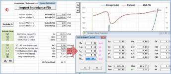
1) Select the type of impedance data file you want to import.
2) Click the [Import Impedance File] Button, browse to the file of interest and select it. The data file is read in, interpolated to LOG spaced data points, “Include” markers are set, and initial values estimates are set for the all the parameters.
3) Click the [LS – fit] to perform the Least Squares fit on the model. Subsequent clicks may improve the fit slightly.
4) The resulting semi-inductance parameters can then be transferred by hand to modeling programs like Hornresp. If significant semi-inductance is present, you may notice the Qes and Qms parameters are a little different than what you had been using and should be transferred as well.
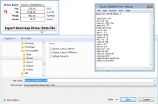
5) Alternatively, you can export an ASCII driver data file to Hornresp. This requires supplying values for Vas, Sd, Pmax, and Xmax. Save the *.txt file in the Hornresp Driver folder.
6) From Hornresp File menu, select the “Paste Driver from Database” function to import the driver data file you just created.
Depending on the quality of the measured data, the steps above may be all you ever need to do. You will notice the upper “Include” marker is set at 10kHz after import. In most cases, this provides better fit in the lower more relevant frequencies, but you can move it as desired. For free-air data measured where the woofer was not firmly clamped, it may be necessary to use the “Exclude” markers to remove the peak of the impedance peak from the LS-fit solution for best fit with the remainder of the curve. In other cases you may find setting some of the parameters by hand and/or removing them from the LS-fit solution (with check boxes) is needed for best fit with measured data.
One thing that is in the works, is the ability to load a second impedance file(closed box or added mass) to calculate Vas. I am also considering adding a tab that could serve as a database of all the drivers you have measured. You could export and share the data as a *.csv file with other users.
Any questions and suggests are welcome.
Attachments
Hi bolserst,
Brilliant work, as always!
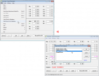
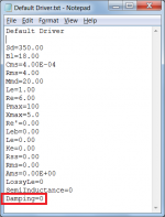
A while ago I changed 'Admittance=' to 'Damping=' in the Hornresp driver data file. My thinking at the time was that because the parameter related to frequency dependent damping, it would most likely be more meaningful to users. I notice that you have used 'Admittance=' in your file, and thinking about it some more, because the value given is in fact an admittance, it would perhaps be better for me to revert back to using that term also. Do you agree?
A small point I know, but I like to get things right") .
.
As far as the actual operation of Hornresp is concerned, it doesn't matter either way.
Kind regards,
David
Brilliant work, as always!
A while ago I changed 'Admittance=' to 'Damping=' in the Hornresp driver data file. My thinking at the time was that because the parameter related to frequency dependent damping, it would most likely be more meaningful to users. I notice that you have used 'Admittance=' in your file, and thinking about it some more, because the value given is in fact an admittance, it would perhaps be better for me to revert back to using that term also. Do you agree?
A small point I know, but I like to get things right
.As far as the actual operation of Hornresp is concerned, it doesn't matter either way.
Kind regards,
David
Attachments
At that vent size you're already into TL-like behaviour when trying to achieve a low Fb, which is why I don't bother with simple vented designs any more.
Simple BR's are boring when we have the marvelous tool HR!
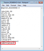
Ooops...I missed the name change in the driver data file.A while ago I changed 'Admittance=' to 'Damping=' in the Hornresp driver data file. ...because the value given is in fact an admittance, it would perhaps be better for me to revert back to using that term also. Do you agree?
To keep names as consistent as possible between the GUI and the driver data file, I would say 'Damping=' is a better choice than 'Admittance='...perhaps 'FDD=' or 'FDDamping=' might be even better.
Attachments
I would say 'Damping=' is a better choice than 'Admittance='...perhaps 'FDD=' or 'FDDamping=' might be even better.
Hi bolserst,
Unfortunately I was in a bit of a hurry yesterday, and not thinking too clearly when I responded to your first post. The reason I changed from 'Admittance=' to 'Damping=' was in fact because the parameter in question stores the on/off status of the frequency-dependent damping option, not an admittance value
.I would prefer to continue using the generic description 'Damping=' though, rather than making a further change to the more specific 'FDD=' or 'FDDamping=' if that is okay with you.
Kind regards,
David
The SPL output and cone excursion is nearly identical between the two, but vent velocity is not.
Hi thejessman,
SPL output is directly related to vent velocity. I can't see how WinISD can have the same output as Hornresp, but a different vent velocity. Something has to be wrong somewhere.
SANITY CHECK:
The radiated power from the port outlet is given by:
Radiated power = [rms volume velocity] ^ 2 * [radiation resistance]
Where:
[rms volume velocity] = Ap * [peak air particle velocity] / Sqrt(2)
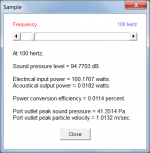
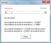
For your example design with resonances masked, radiating into 2 Pi space, at 100 Hz:
Ap = 127.02 cm^2
Peak air particle velocity = 1.0132 m/sec (see Attachment 1)
Radiation resistance = 0.0022 acoustical ohms (see Attachment 2)
In mks units:
Ap = 127.02 *10 ^ -4 m^2
Peak air particle velocity = 1.0132 m/sec
Radiation resistance = 0.0022 * 10 ^ 5 mks acoustical ohms
Rms volume velocity = 127.02 *10 ^ -4 * 1.0132 / Sqrt(2) = 0.0091 m^3/sec
Therefore:
Radiated power = 0.0091 ^ 2 * 0.0022 * 10 ^ 5 = 0.0182 watts
Pressure at 1 metre for 2 Pi radiation:
Pressure = Sqrt([radiated power] * [air density] * [sound velocity] / [hemispherical surface area])
Pressure = Sqrt(0.0182 * 1.205 * 344 / (2 * Pi)) = 1.0958 Pa
SPL = 20 * Log10 (Pressure / Pref) = 20 * Log10 (1.0958 / (20 * 10 ^ -6)) = 94.77 dB
CONCLUSION:
The 94.77 dB result above is the same as the SPL figure given in Attachment 1, only in this case it has been calculated using the Hornresp value for port outlet air particle velocity, rather than the method by which SPL is normally calculated. As can be seen from the above example, the Hornresp results are entirely consistent.
If WinISD has a lower value for air particle velocity, then the WinISD SPL should be lower also, if the calculations are being done correctly. The WinISD results are seemingly not consistent.
Kind regards,
David
Attachments
Hi Orion33,
It is the straight-line distance between the centres of the driver and port, measured on the front panel.
In all cases the driver and port are treated as point sources. Specify the straight-line distance between the centres of the two outputs.
It is not possible to calculate the combined pressure response without knowing the directivity characteristics of the two sources and their positions relative to the listener.
Kind regards,
David
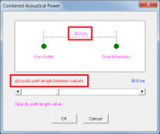
1. What means "acoustic path length" parameter? Is it distanse between axises of driver and port measured on front panel? Or is it depth between surfaces?
It is the straight-line distance between the centres of the driver and port, measured on the front panel.
2. How to simulate cases when driver and port are in different surfaces?
In all cases the driver and port are treated as point sources. Specify the straight-line distance between the centres of the two outputs.
3. And about power responce again. I already asked this question: http://www.diyaudio.com/forums/subwoofers/119854-hornresp-784.html#post5180117
It is not possible to calculate the combined pressure response without knowing the directivity characteristics of the two sources and their positions relative to the listener.
Kind regards,
David
Thank you for answers, David.
OK, and where is virtual microphone in both cases?It is the straight-line distance between the centres of the driver and port, measured on the front panel.
In all cases the driver and port are treated as point sources. Specify the straight-line distance between the centres of the two outputs.
But how does Martin J. King calculate SPL?It is not possible to calculate the combined pressure response without knowing the directivity characteristics of the two sources and their positions relative to the listener.
Hi Orion33,
Pressures are calculated at a point 1 metre from the centre of each of the two sound power sources, taking into account the solid radiation angle. The resultant combined pressure is then determined, taking into account the differences in level and volume velocity phase of each source, and the acoustic path length between the two sources as specified by the user. The resultant combined pressure is then converted to SPL.
Presumably assumptions are made regarding the directivity of the combined system. The directivity of a piston in an infinite baffle is sometimes used to provide an indicative pressure response, but this approach has its limitations and the high-frequency results can become quite inaccurate, particularly when horn loudspeakers are involved. I guess you would really need to ask Dr King what he does, to know for sure.
Kind regards,
David
OK, and where is virtual microphone in both cases?
Pressures are calculated at a point 1 metre from the centre of each of the two sound power sources, taking into account the solid radiation angle. The resultant combined pressure is then determined, taking into account the differences in level and volume velocity phase of each source, and the acoustic path length between the two sources as specified by the user. The resultant combined pressure is then converted to SPL.
But how does Martin J. King calculate SPL?
Presumably assumptions are made regarding the directivity of the combined system. The directivity of a piston in an infinite baffle is sometimes used to provide an indicative pressure response, but this approach has its limitations and the high-frequency results can become quite inaccurate, particularly when horn loudspeakers are involved. I guess you would really need to ask Dr King what he does, to know for sure
.Kind regards,
David
I'm confussed. Before, you said that you plot acoustical power instead SPL. Then you told that straight-line distance between the centres of the driver and port, measured on the front panel. And so I thought, that virtual microphone, that measured combo responce, is placed somewhere on front panel. So I asked - where? This can be on the axis of the driver, on the axis of the port or on the normals drawn through middle of the acoustic path.Pressures are calculated at a point 1 metre from the centre of each of the two sound power sources, taking into account the solid radiation angle. The resultant combined pressure is then determined, taking into account the differences in level and volume velocity phase of each source, and the acoustic path length between the two sources as specified by the user. The resultant combined pressure is then converted to SPL.
Hi Orion33,
The "acoustic path length" is the direct straight-line distance separating the two sound outputs, it is not the distance to the listener or virtual microphone. The Hornresp simulation model performs a radiated power summation of two spaced point sources. The pressure is then calculated at a distance of 1 metre from an equivalent single point source that radiates the summed acoustical power. As far as the model is concerned, because the power is being radiated uniformly in all directions from a point source, constrained only by the specified solid radiation angle, the position of the virtual microphone can be anywhere inside the solid angle, provided that the distance from the microphone to the point source remains at 1 metre.
Kind regards,
David
Attachments
Where is this source located? If this is just algebraic addition of acoustic powers from two point sources, then this sum will not depend on the distance between them. Because each is calculated independently of another source each time. Since the graph of the sum varies depending on this distance, I assume that this is an acoustic sum that takes into account the geometry. I would like to know where is this virtual source.The pressure is then calculated at a distance of 1 metre from an equivalent single point source that radiates the summed acoustical power.
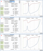
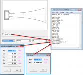
I think these pictures will help understand the question of what I mean

In the first case, the driver and port are located on the front side. The distance between their axes corresponds to your definition in the program. We calculate the response at 1 m from the middle or somewhere else there.
In the second picture, the same response will be at the green point. But I'm interested in receiving the response in the same black point. Obviously, it will be different, because the acoustic path from the port to the black point has increased (bold blue line).
Where to crossover a subwoofer(highest possible frequency)
Hi,
assuming i built a subwoofer with this frequency response:
What's the highest frequency where a passive 12db/Octave 2-way crossover may have the crossover-point?
I mean, whats the real life experience, as there may be more dampening effect on the peak at 300Hz from the neclosure walls, and maybe other things ...
Thanks,
Johannes
Johannes
Hi,
assuming i built a subwoofer with this frequency response:
An externally hosted image should be here but it was not working when we last tested it.
.png)
What's the highest frequency where a passive 12db/Octave 2-way crossover may have the crossover-point?
I mean, whats the real life experience, as there may be more dampening effect on the peak at 300Hz from the neclosure walls, and maybe other things ...
Thanks,
Johannes
Johannes
That image looks familiar...
A few things:
1. It is not a subwoofer. Calling a bass module with a 48 Hz Fb a "subwoofer" is stretching the term a little bit.
2. An 80~100 Hz x-over point should be fine with that build. You can go higher with a sharper x-over (24dB/oct LR is what I'd recommend).
3. The Hornresp sim assumes an unfolded TL. Folds will introduce some response variations and act as LP filters at frequencies that depend on the size of the fold. The response will likely have only a vague resemblance to the SIM @300 Hz because around that frequency the folds will begin to affect the response from the vent and therefore the overall response. I never measured it that high @ 1M or further because I had no intention of using it that high, however I could arrange to do so if you're interested.
Sounds fine to me....I would prefer to continue using the generic description 'Damping='...
I will update the export code of the Semi-Le spreadsheet in the next update.
- Home
- Loudspeakers
- Subwoofers
- Hornresp