(Thread title inspired by @Boden from @bwaslo's thread "Xsim-3D development... I could use some math help")
A little background first: I've done many loudspeaker measurements with the tool set that many DIYers have, a calibrated mic and some free software, but I'm looking for a better system. I've been looking more closely at Earl Geddes measurement method, and Gabriel Weinreich's paper "Method for measuring acoustic radiation fields" and what I can find on the function of Klippel's Near Field Scanner. Bwaslo's recent thread "Xsim-3D development... I could use some math help" took a turn that made me want to start getting some help on understanding all this. And like Bill's thread, I could use some math help...
In addition, a number of very interesting questions were rasied to Earl Geddes about more advanced measurement methods that I think could use their own thread.
So so far, I have two big questions I'd like some help with, please:
1. what is needed to turn a measurement set into a view of radiation modes (for lack better way to ask the question)? Geddes uses a FORTRAN routine, but would something like open source mathematical software work, or is it best to have purpose built software?
2. Weinreich's paper and the Near Field Scanner both are capable of "sound field separation", in other words, they can pull the room reflections out of the measurement and give you just the direct sound from the speaker (no need for an anechoic chamber!). Klippel only appears to do this up to 1kHz (plus or minus an octave) and uses measurement windowing above that, Weinreich didn't appear to us it very high in frequency either. It appears to work by looking at the timing of sound waves passing through a pair of measurement shells? But what I'd really like to know is if Weinreich could do that with technology from the late 1970's, can intrepid DIYers do the same with available software and hardware today?
And please, if anyone else has questions about the function of more advanced speaker measurement systems, please post them here.
... Earl Geddes measurement method, and Gabriel Weinreich's paper ...
Nice project, have you seen >this< paper?
It includes some newer references that may be useful, I haven't read them yet.
Best wishes
David
Last edited:
That is a good paper, precisely what I am talking about.
I originally did my analysis in MathCad, but it was painfully slow. When I rewrote it in FORTRAN with a VB.net interface it was virtually instantaneous. So purpose build software does have significant advantages.
Weinreich's technique would require custom software as there is no existing software that can do this (short of Klippel.)
To me the best idea is to start simple and build from there, especially if DIY is the goal. Jumping into a full Klippel level of analysis is bound to fail for anyone without his resources. I started with horizontal only for just this reason - it is much simpler than a general purpose analysis. I also did not use the two surface technique and just use gating. Various techniques were used at the low end were the window effect was detrimental.
What should be noteworthy here is that my system, simple as it was, has been extremely effective at allowing me to push ever more sophisticated designs. So much so, that I simply kept the entire concept to myself for many many years (heck the Weinreich paper is decades old!!) It was a competitive advantage. But I no longer make speakers and so it seems to me that disseminating the technology would be a good gift to the audio community. So any participation of mine has to be for "Open access". "Open Source" is not a requirement as long as the DIY community has free access to the software.
At this point, a scanning array seems like over-kill to me. Much better to start as I started and go simple. Do the horizontal and then with a few measurements above and below the horizontal plane one can add in the vertical holes from the crossover. To me this is what a DIY needs, not the full 3D that Klippel does for Pro Sound applications (which really do need full 3D, and probably can afford 20k$.)
Nice project, have you seen >this< paper?
It includes some newer references that may be useful, I haven't read them yet.
Best wishes
David
Thank you David, hopefully the project comes to something useful! I will give that paper and references a read. It looks like it will be helpful, thank you.
That is a good paper, precisely what I am talking about.
I originally did my analysis in MathCad, but it was painfully slow. When I rewrote it in FORTRAN with a VB.net interface it was virtually instantaneous. So purpose build software does have significant advantages.
Weinreich's technique would require custom software as there is no existing software that can do this (short of Klippel.)
To me the best idea is to start simple and build from there, especially if DIY is the goal. Jumping into a full Klippel level of analysis is bound to fail for anyone without his resources. I started with horizontal only for just this reason - it is much simpler than a general purpose analysis. I also did not use the two surface technique and just use gating. Various techniques were used at the low end were the window effect was detrimental.
What should be noteworthy here is that my system, simple as it was, has been extremely effective at allowing me to push ever more sophisticated designs. So much so, that I simply kept the entire concept to myself for many many years (heck the Weinreich paper is decades old!!) It was a competitive advantage. But I no longer make speakers and so it seems to me that disseminating the technology would be a good gift to the audio community. So any participation of mine has to be for "Open access". "Open Source" is not a requirement as long as the DIY community has free access to the software.
At this point, a scanning array seems like over-kill to me. Much better to start as I started and go simple. Do the horizontal and then with a few measurements above and below the horizontal plane one can add in the vertical holes from the crossover. To me this is what a DIY needs, not the full 3D that Klippel does for Pro Sound applications (which really do need full 3D, and probably can afford 20k$.)
As I've been thinking about this project over the last month or so, I had been heading to the conclusion that it would be best to start with a simple system rather than a full scanning array. Although I would like to get to that point somewhere down the road.
Would it be possible to obtain a copy of the MathCAD routine you used? If you'd rather not, that's quite alright. Basically, I'm looking for a starting point, so any kind of direction about how to get there would be most helpful.
In the other thread, you mentioned (link):
Do understand this correctly, that if a setup like yours had very accurate mic placement, the measurements could be made in the near-field, or was this in reference to 3D scanning microphone? Because the prospect of having such a high signal to noise ratio is certainly motivating to design a device that can place a mic that precisely.Finally, one does not even have to be in the far field to do this (in the spherical case) and Klippel does it very close to the source, but this requires very accurate placement of the mic, hence the $20,000 price tag. I back up to 1-1.5 meters and positioning is not so important. Once you have the source velocities you have all the field data, all angles and all radii, even near field.
Thank you for the assistance so far, sharing this information is certainly a superb gift to the audio community. After all, the clearer we can see what a speaker is doing, the better speaker we can make.
...that paper and references a read. It looks like it will be helpful, thank you.
Just a "heads up" -
A closer look at the references reveals that some of the ones I considered new seem to be incorrect citations of old ones.
The Chinese use different name conventions and I suspect that's why they have messed them up.
Still a few references were new to me however.
...the conclusion that it would be best to start with a simple system...
I was about to recommend that too
")
Just a pivoted arm to scan the horizontal plane at first?
Even make it manual, not too many points if it's only in one plane.
Once you can transform that data then add a stepper motor to automate rotation, with manual Z axis.
Then add Z axis automation if it all works.
I can try to help with the maths, I needed to revise Bessel functions anyway
Best wishes
David
On a practical setup aspect - I've never understood why the Klippel system uses only 1 microphone and has a complex extra mechanics to move that one microphone back and forth to 2 distances. Most analyzers will have at least a inputs and getting two reasonable good microphones is also not such a big problem. So to me it seems to be a better idea to use 2 mics at 2 distances. Additional benefit is to get 2 points measured with same sweep run per horizontal rotation angle.
Would it be possible to obtain a copy of the MathCAD routine you used?
Do understand this correctly, that if a setup like yours had very accurate mic placement, the measurements could be made in the near-field, or was this in reference to 3D scanning microphone? Because the prospect of having such a high signal to noise ratio is certainly motivating to design a device that can place a mic that precisely.
I'll try and dig up a Mathcad routine, although I haven't done it that way in more than ten years. Still, it will give you an idea of how I came to what I do now, it's a good start.
In theory it matters not how close one gets to the system as long as the spherical surface that you scan completely contains the DUT. However, I have never tested that out. I usually use 1.5 meters as this gives me a decent window for data above 200 Hz. Below 200 Hz I use a different technique which works well for a closed box - like all my speakers are - but not as well for ported and dipoles. SNR tends to not be an issue because the fitting routines are robust to noise in the data. Clearly you have to have only the direct sound as that's the biggest concern.
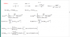
OK, I finally found the Mathcad files. I have attached them (not the full files just pages, the full files are dozens of pages.)
Note:
1)any name with "fft" in it is FFT data.
2) there are two drivers, "high" and "low"
3) the integral at the bottom does all the rest of the work
4) "coef_) is an array of modal coefficients by FFT frequency
5) the function Leg(n,x) is a mathcad function of the legendre polynomials of order "n" in "x"
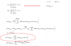
On the other posting:
1) The circled line contains the reconstruction from modal back to SPL data for plotting in a polar map where "iplot" is the smoothed frequency by "it" the field angle
Remember this was the first step and these pages are simplifications of what I ended up doing, but if you can follow this you will see that the basics are pretty simple
The printout is hard to follow, I can't even remember what it all is doing.
Note:
1)any name with "fft" in it is FFT data.
2) there are two drivers, "high" and "low"
3) the integral at the bottom does all the rest of the work
4) "coef_) is an array of modal coefficients by FFT frequency
5) the function Leg(n,x) is a mathcad function of the legendre polynomials of order "n" in "x"
On the other posting:
1) The circled line contains the reconstruction from modal back to SPL data for plotting in a polar map where "iplot" is the smoothed frequency by "it" the field angle
Remember this was the first step and these pages are simplifications of what I ended up doing, but if you can follow this you will see that the basics are pretty simple
The printout is hard to follow, I can't even remember what it all is doing.
Attachments
Last edited:
Apologies for taking so long to get back to this, I’ve been traveling and haven’t had an opportunity to respond.
And I would very much appreciate some help with the math. I’ll send you a PM soon.
Question (possibly a dumb one) about note 2: what are the drivers “high” and “low” are referring to?
Thanks for the heads up. I did track down a few of them.Just a "heads up" -
A closer look at the references reveals that some of the ones I considered new seem to be incorrect citations of old ones.
The Chinese use different name conventions and I suspect that's why they have messed them up.
Still a few references were new to me however.
Exactly! That is pretty much the set-up that I had been thinking about to start with. I figure that once I understand the math better and there’s a working measurement system, then I can start working toward the full 3D/field separation setup.Just a pivoted arm to scan the horizontal plane at first?
Even make it manual, not too many points if it's only in one plane.
Once you can transform that data then add a stepper motor to automate rotation, with manual Z axis.
Then add Z axis automation if it all works.
I can try to help with the maths, I needed to revise Bessel functions anyway
And I would very much appreciate some help with the math. I’ll send you a PM soon.
I assume that they use a single microphone to guarantee the same phase/amplitude response for each measurement point. Nevertheless, Weinreich's method used two microphones, and given how many points need to be taken, reducing measurement time would certainly be nice.On a practical setup aspect - I've never understood why the Klippel system uses only 1 microphone and has a complex extra mechanics to move that one microphone back and forth to 2 distances. Most analyzers will have at least a inputs and getting two reasonable good microphones is also not such a big problem. So to me it seems to be a better idea to use 2 mics at 2 distances. Additional benefit is to get 2 points measured with same sweep run per horizontal rotation angle.
Good to know. I’d be interested to explore that if this project progresses. I recall that in Klippel’s literature it is stated that the scan surface radius depends on the size of the DUT. Presumably to keep the direct sound level as high as possible. Since that is (at least theoretically) true, In addition to speakers, I can see having a setup like this for raw driver measurements would be very useful.In theory it matters not how close one gets to the system as long as the spherical surface that you scan completely contains the DUT. However, I have never tested that out
Thank you! That is very helpful; it’ll take some time to digest.OK, I finally found the Mathcad files. I have attached them (not the full files just pages, the full files are dozens of pages.)
Note:
1)any name with "fft" in it is FFT data.
2) there are two drivers, "high" and "low"
3) the integral at the bottom does all the rest of the work
4) "coef_) is an array of modal coefficients by FFT frequency
5) the function Leg(n,x) is a mathcad function of the legendre polynomials of order "n" in "x"
On the other posting:
1) The circled line contains the reconstruction from modal back to SPL data for plotting in a polar map where "iplot" is the smoothed frequency by "it" the field angle
Remember this was the first step and these pages are simplifications of what I ended up doing, but if you can follow this you will see that the basics are pretty simple
The printout is hard to follow, I can't even remember what it all is doing.
Question (possibly a dumb one) about note 2: what are the drivers “high” and “low” are referring to?
This page is from a calculation of a two driver system where there is a crossover. Hence high is the tweeter and low is the woofer. This technique allowed me to generate the entire polar map from individual driver measurements which included the crossover. Not a trivial task, but made much easier by the modal expansion.
@Dave Zan... your inbox is full.
My DIY profile "About Me" tab has my email address, more space than the DIY inbox.
Sorry for any inconvenience, can you resend it?
Best wishes
David
I'm now thinking about releasing my PolarMap software for general use by rewriting it to make it more like something of added value instead of just a PITA.
It dawned on my that some public input might be useful. I use Holm Impulse to take data as this is an extremely robust piece of software that is free, but as with any software its data files ha a specific format. I might entertain other measurement packages, but using Holm will be first as that already works well. Is there a second choice or a data format choice for a future enhancement?
It dawned on my that some public input might be useful. I use Holm Impulse to take data as this is an extremely robust piece of software that is free, but as with any software its data files ha a specific format. I might entertain other measurement packages, but using Holm will be first as that already works well. Is there a second choice or a data format choice for a future enhancement?
No problem at all! Email sent, thanks for your help.My DIY profile "About Me" tab has my email address, more space than the DIY inbox.
Sorry for any inconvenience, can you resend it?
Best wishes
David
I'm now thinking about releasing my PolarMap software for general use by rewriting it to make it more like something of added value instead of just a PITA.
It dawned on my that some public input might be useful. I use Holm Impulse to take data as this is an extremely robust piece of software that is free, but as with any software its data files ha a specific format. I might entertain other measurement packages, but using Holm will be first as that already works well. Is there a second choice or a data format choice for a future enhancement?
It would certainly be an added value. My observation is that DIY'ers who I would consider to be serious about making a good design typically measure at 10 degree increments, and are at least aware that finer angular resolution would be better. But I think most of them are like me: starting from scratch learning the programming and math. So I'm sure they would all greatly appreciate a tool that gives them more detail for less work. Even those that aren't as serious can surly see the benefits.
As far as other data format choices, Room EQ Wizard might be the most popular freeware measurement software right now. Although if I'm remembering, you export the measurements from Holm Impulse into .txt files to import into PolerMap, and Room EQ Wizard can export a measurement set as .txt. But along those lines, in addition to .txt, .frd seems to be a pretty common data format for DIY audio measurements.
FRD files have already been windowed and the windowing should be done in my program. So what I need are impulse response files. If REW can export a measurement set as impulse responses into a *.txt file then that's ideal. If you have such a file could you send it to me so that I can see its format.
It doesn't look like REW can do a batch export of IR to .txt, but it can do individual measurement one at a time, which is a bit tedious.
I have attached two sets I have. As heads up; they are ten degree angular resolution and only out to 90 degrees. It's all I had for existing measurements, although I remember doing a set once with the angles that you use. I can try to dig it up if that would be better. I attached two measurement sets because I know that Holm deals with timing references different than REW, so one (MA1 IR) uses a loopback timing reference and the other does not.
Edit: looks like the files are too big to attach here. Do you have a preferred way that I can send them to you?
Last edited:
FRD files aren't inherently windowed, the data can be windowed or unwindowed. But it is frequency domain rather than time domain (an IFFT can turn it around of course). FRD is almost not a format, it's just a text list of frequency, dB level (acoustic or electric) and phase, space or tab separated on each line and a line return after each line. The only hard requirement is that the frequencies be in ascending order and anything that starts without a frequency at the first character of a line should begin with a letter or punctuation (quote mark preferred) and all happen before the actual data starts. Pretty much the most simple and obvious way to relate a general frequency response curve
...my PolarMap software...
The Klippel scanner software shows "the whole catastrophe" of spherical harmonics.
The Mathcad extract you posted previously calculates just the azimuth polar, which needs only the simpler Legendre polynomials.
Your notes to PolarMap also discuss this choice.
I would like to follow your wise advice (and my own recommendation to the OP) and start simple.
Simplest of all is uniformly spaced measurements, but I note you take yours closer near the main axis.
That seems intuitively reasonable, how does it work out in the maths?
Best wishes
David
I had a closer look at Bill Waslo's Xsim-3d thread and found some info there.
More details still welcome.
Last edited:
- Home
- Design & Build
- Software Tools
- Klippel Near Field Scanner on a Shoestring