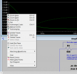
Right-click the Y axis and select Logarithmic or Linear. When the scale is in db LTSpice omits the unit name.
You can also right-click on the name of the trace at the top of the plot and then enter in your equation. That's usually faster then going through the "add trace" dialogue.
You can also right-click on the name of the trace at the top of the plot and then enter in your equation. That's usually faster then going through the "add trace" dialogue.
 I can play about with this now.
What I want to do is plot impedance as a graph... and I'm struggling with this.
So how is that done please ?")
Use a current source
Attachments
Use a current source
In the current source sample, try the different plots 'V(vout)/1' and 'V(vout)/1A' (the second formula gives the result in Ohm's, no need to change any settings)
My first method only works for DC, your scheme has a capacitor in series this makes the DC impedance infinite (or there about ). When there is a DC path I always (most of the time) use the method I published first. Both methods have there usage, and the different results they give are (at the least to me) of great interest!
http://www.diyaudio.com/forums/soft...ng-ltspice-beginner-advanced.html#post4128856
http://www.diyaudio.com/forums/soft...ng-ltspice-beginner-advanced.html#post4129181
). When there is a DC path I always (most of the time) use the method I published first. Both methods have there usage, and the different results they give are (at the least to me) of great interest! http://www.diyaudio.com/forums/soft...ng-ltspice-beginner-advanced.html#post4128856
http://www.diyaudio.com/forums/soft...ng-ltspice-beginner-advanced.html#post4129181
Even at 1000meg and it still runs OK...
Ahhh, the 1TV (and even more) solution (1TV = 1.000.000.000.000,00 Volts
)Measuring amplifier output impedance.
Thanks to FdW and keantoken I now know how to get the Y axis to display the apparent Z out in "ohms" and I think I understand using the "current" method rather than the "voltage method" to derive a value for Zout. In some very quick trial runs they seem to produce identical results. Next step is to put some different values into the circuit and try and prove it works by calulating it out as a check.
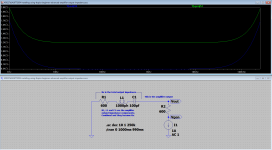
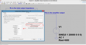
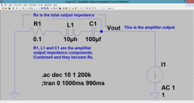
So here is the new circuit. The voltage source has been replaced with a current source (that is selectable in the standard LT parts section). The only changes are that the 600 ohm resistor that was unrealistically high for an amplifier output impedance is now a more reasonable 0.1 ohms and the inductor is now 10uh. I'm leaving the cap as 100uf at this stage as it makes for a nice simulation. The "AC Analysis" has now been changed to cover 1Hz to 200kHz and because we are using a current source, the series backfeed resistor has been omitted.

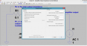
And the settings for AC Analysis. Even though this is now a current source we have similar options to the more familiar voltage source.

We can now run the sim and enter our expression to calculate Zout. Zout at any given frequency is Zout = Vout/IR1. That is because the current that flows in R1 is what develops the voltage across the amplifiers internal output impedance and we see that as Vout. Knowing those two variables we can work out what the unknown series amplifier output impedance must be. What we are plotting is that calculation, and displaying the result in ohms on the Y axis together with frequency on the X axis.
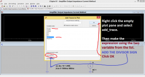
So we run the sim but this time we do not probe Vout, we right click the empty "plot pane" and select "new trace". Pick Vout and IR1 from the list making sure the divisor sign is added. Then click OK.

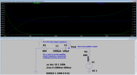
You should now see a plot that looks like this. What we need to do though is to change the units at the left into ohms (Thanks keantoken)

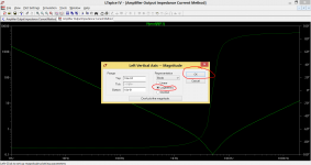
If you now move the cursor to the left of the screen (over the Y axis) you will see it change to a ruler symbol. Left click and select "logarithmic". Also make sure that "Bode" is selected as default. When you click OK the units at the left should change to ohms.
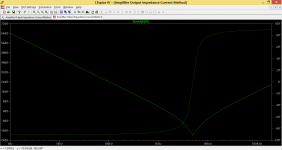
Now you should hopefully see this. Notice how the impedance dips to a minimum of around 0.1 ohms at around 5kHz. Below this point, the effect of the 100uf cap is dominant and causes the expected LF roll off. Above and the inductor comes into play causing HF roll off. However its a little more complicated than than that, and I want to go on and try and "prove" the results.

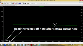
This is now the point I wanted to do a quick check by working it all out long hand I have picked two frequencies of interest, 100Hz and 20kHz. If we run the sim and look at the graph, we can, by mousing over those two points on the curve, read off the impedance. Don't try and read the graph directly, use the numerical readout at the bottom left of the screen. Here is a shot with the area around 100Hz zoomed in up close and the values shown at the bottom.

I make the values around 15.6 ohm and 1.18 ohm respectively. Now to prove it by calculation and also by reconfiguring the sim to something more familiar as a double check.
Firstly we need to calculate XL and XC using the standard formulas for reactance (2piFL and 1/2piXC) for the two frequencies we have chosen.
XL = 0.0063 ohm and XC = 15.9 ohm at 20Hz
XL = 1.25 ohm and XC = 0.08 ohm at 20kHz
R is a constant of course at 0.1 ohm.
The total impedance of a series network consisting of one cap, one inductor and one resistor is given by the formula Z= √(R*R) + (XL-XC)^2. In English that means taking multiplying R by itself and then and adding whatever the result of XL minus XC squared is. Then finally find the square root of that number.
Lets do it For 100Hz we get 15.9 ohm. There are the inevitable rounding errors in the calculation but that compares very well with the 15.9 ohm read from the graph.
For 20kHz we get 1.17 ohm which also compares well with the 1.18 I read from the graph. All good. Really good. (wow... I'm pleased that worked haven't done that since I was at technical college)
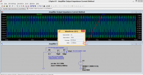
We can run another check that brings us back to more familiar territory. If we set the sim up again but this time with a voltage source together with its series resistor we can simply read off the RMS current in the series backfeed resistor and also the RMS voltage at the amplifier output. Remember to set
the voltage source to the frequency required, 100Hz and 20kHz in this case and to change the sim type to "transient". For 20kHz we get a current 1.1545ma RMS in R2 and a voltage 1.364 vRMS at the output. Z= V/I which is 1.18 ohm.

Here it is set for 20kHz with the source current and output voltage displayed. Notice how I have added the 600 resistor directly into the voltage source as a series impedance.

So all methods seem to be giving the correct values which is really good.
There is one more thing we can confirm by calculation and that is the resonant frequency of the reactive part of the output impedance. If you look at the
graph you will see it dips to a minimum value around 5kHz. What actually is that though ? Well it is the resonant frequency of the R/C/L component of the
output impedance. As a check we can calculate that by using the formula Fr = 1/2pi√L*C (in English, 1 over two pi root LC) Putting the numbers in and we get 5032Hz.
The .asc file attached is setup with the current source method.
Thanks to FdW and keantoken I now know how to get the Y axis to display the apparent Z out in "ohms" and I think I understand using the "current" method rather than the "voltage method" to derive a value for Zout. In some very quick trial runs they seem to produce identical results. Next step is to put some different values into the circuit and try and prove it works by calulating it out as a check.
So here is the new circuit. The voltage source has been replaced with a current source (that is selectable in the standard LT parts section). The only changes are that the 600 ohm resistor that was unrealistically high for an amplifier output impedance is now a more reasonable 0.1 ohms and the inductor is now 10uh. I'm leaving the cap as 100uf at this stage as it makes for a nice simulation. The "AC Analysis" has now been changed to cover 1Hz to 200kHz and because we are using a current source, the series backfeed resistor has been omitted.
And the settings for AC Analysis. Even though this is now a current source we have similar options to the more familiar voltage source.
We can now run the sim and enter our expression to calculate Zout. Zout at any given frequency is Zout = Vout/IR1. That is because the current that flows in R1 is what develops the voltage across the amplifiers internal output impedance and we see that as Vout. Knowing those two variables we can work out what the unknown series amplifier output impedance must be. What we are plotting is that calculation, and displaying the result in ohms on the Y axis together with frequency on the X axis.
So we run the sim but this time we do not probe Vout, we right click the empty "plot pane" and select "new trace". Pick Vout and IR1 from the list making sure the divisor sign is added. Then click OK.
You should now see a plot that looks like this. What we need to do though is to change the units at the left into ohms (Thanks keantoken
)
If you now move the cursor to the left of the screen (over the Y axis) you will see it change to a ruler symbol. Left click and select "logarithmic". Also make sure that "Bode" is selected as default. When you click OK the units at the left should change to ohms.
Now you should hopefully see this. Notice how the impedance dips to a minimum of around 0.1 ohms at around 5kHz. Below this point, the effect of the 100uf cap is dominant and causes the expected LF roll off. Above and the inductor comes into play causing HF roll off. However its a little more complicated than than that, and I want to go on and try and "prove" the results.
This is now the point I wanted to do a quick check by working it all out long hand
I have picked two frequencies of interest, 100Hz and 20kHz. If we run the sim and look at the graph, we can, by mousing over those two points on the curve, read off the impedance. Don't try and read the graph directly, use the numerical readout at the bottom left of the screen. Here is a shot with the area around 100Hz zoomed in up close and the values shown at the bottom.
I make the values around 15.6 ohm and 1.18 ohm respectively. Now to prove it by calculation and also by reconfiguring the sim to something more familiar as a double check.
Firstly we need to calculate XL and XC using the standard formulas for reactance (2piFL and 1/2piXC) for the two frequencies we have chosen.
XL = 0.0063 ohm and XC = 15.9 ohm at 20Hz
XL = 1.25 ohm and XC = 0.08 ohm at 20kHz
R is a constant of course at 0.1 ohm.
The total impedance of a series network consisting of one cap, one inductor and one resistor is given by the formula Z= √(R*R) + (XL-XC)^2. In English that means taking multiplying R by itself and then and adding whatever the result of XL minus XC squared is. Then finally find the square root of that number.
Lets do it
For 100Hz we get 15.9 ohm. There are the inevitable rounding errors in the calculation but that compares very well with the 15.9 ohm read from the graph.For 20kHz we get 1.17 ohm which also compares well with the 1.18 I read from the graph. All good. Really good. (wow... I'm pleased that worked
haven't done that since I was at technical college)We can run another check that brings us back to more familiar territory. If we set the sim up again but this time with a voltage source together with its series resistor we can simply read off the RMS current in the series backfeed resistor and also the RMS voltage at the amplifier output. Remember to set
the voltage source to the frequency required, 100Hz and 20kHz in this case and to change the sim type to "transient". For 20kHz we get a current 1.1545ma RMS in R2 and a voltage 1.364 vRMS at the output. Z= V/I which is 1.18 ohm.
Here it is set for 20kHz with the source current and output voltage displayed. Notice how I have added the 600 resistor directly into the voltage source as a series impedance.
So all methods seem to be giving the correct values which is really good.
There is one more thing we can confirm by calculation and that is the resonant frequency of the reactive part of the output impedance. If you look at the
graph you will see it dips to a minimum value around 5kHz. What actually is that though ? Well it is the resonant frequency of the R/C/L component of the
output impedance. As a check we can calculate that by using the formula Fr = 1/2pi√L*C (in English, 1 over two pi root LC) Putting the numbers in and we get 5032Hz.
The .asc file attached is setup with the current source method.
Attachments
-
 RMS Values.PNG124.5 KB · Views: 207
 -
 Volt Check.PNG54.7 KB · Views: 211
 -
 Readout.png170.8 KB · Views: 204
 -
 Plot 2.PNG43.7 KB · Views: 201
 -
 Plot 1.PNG33.4 KB · Views: 198
 -
 Enter Expression.PNG75.9 KB · Views: 199
 -
 AC Impedance Analysis.PNG53.1 KB · Views: 208
 -
 New Output Impedance Circuit.PNG45.3 KB · Views: 214
 -
Amplifier Output Impedance Current Method.asc1.2 KB · Views: 190
@Mooly,
Would you know of a way to use the .step param to gauge a certain component's effect on THD? Ideally I'd like to arrive at a single THD20K value for each value in the .step param list. This would allow me, and I'm sure others, to quickly converge to an optimum, rather than having to make each run individually.
Would you know of a way to use the .step param to gauge a certain component's effect on THD? Ideally I'd like to arrive at a single THD20K value for each value in the .step param list. This would allow me, and I'm sure others, to quickly converge to an optimum, rather than having to make each run individually.
I'm not quite sure where the problem is ... if you know how to use the .step param, and add a .four directive to the schematic, then the SPICE error log automatically shows the THD figures for each run, one following the other ...@Mooly,
Would you know of a way to use the .step param to gauge a certain component's effect on THD? Ideally I'd like to arrive at a single THD20K value for each value in the .step param list. This would allow me, and I'm sure others, to quickly converge to an optimum, rather than having to make each run individually.
@Mooly,
Would you know of a way to use the .step param to gauge a certain component's effect on THD? Ideally I'd like to arrive at a single THD20K value for each value in the .step param list. This would allow me, and I'm sure others, to quickly converge to an optimum, rather than having to make each run individually.
If it's a resistor, you can give it the value of a simulation parameter by putting {var} in it's value box where var is a variable defined by the simulator directive:
.param var=100
The value of the resistor will be 100 then. Next you can use the .step command to step through a number of preset values:
.step param var list 66.9 82 99.3 133
The simulator will repeat 4 times changing the value of the resistor to each value listed successively. If you look at the LTspice help file you can read about doing logarithmic or linear steps with the .step command as well. You can do this for any component, E sources, voltage sources, resistors, capacitors...
You can even do this with transistors if you're clever. For instance change the name of the transistor (Rclick on the transistor name, not the transistor symbol) to {mod}, and then make a bunch of doppleganger models to step through:
.param mod=1
.step param mod list 1 2 3 4
.model 1 AKO:BC550C_C
.model 2 AKO:BC337-40_kq
.model 3 AKO:2N5551_C
The simulation will repeat using each transistor successively.
You can even take advantage of this to make stepped simulations using a unique bias value for each transistor. For instance:
.param Rbias=110.3
.step param Rbias list 110.3 112 113.6
.model 110.3 AKO:BC550C_C
.model 112 AKO:BC337-40_kq
.model 113.6 AKO:2N5551_C
Then you use {Rbias} in the value box for the bias resistor, and also for the name of the transistor(s) you want to change.
And if you really want to get fancy - and sometimes this is precisely what is needed - you can use the "table" function to vary any number of parameters in the schematic for each run ... say, change the whole set of active devices in various combinations, to see what happens.
- Home
- Design & Build
- Software Tools
- Installing and using LTspice IV (now including LTXVII), From beginner to advanced