OK, here's the circuit,
If anyone could contribute to this it would be much appreciated. I'm trying to keep this really simple and explain every step I take here.
So here we have the circuit set up for an output of 1 watt rms into 8 ohm. How would you set up a simulation to find a realsitic THD value for this ?
The settings I am using are these,
.op
.option noopiter (because the simulator can not find an operating point using the default method and the error log suggests adding this directive)
.option plotwinsize=0
.maxstep=0.488331106u I've read up on this and how to calculate the value (I think") )
)
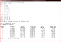
.four 1khz 10 4 v(vout) I understand that looks at the first 10 harmonics over the last four cycles.
.tran 8m
The input signal is 1khz for 16 cycles at a level that gives 1 watt rms output. So I run the simulation and get the following THD report showing 0.0011%.
So first question... is there any problem in the settings used so far to derive that figure ?
-----------------------------------------------------------------------------------------------------------------------------------------
Next part of the question...
The figures in the THD print out seem to be the figures that really matter. The FFT plot which I'll come to next can be made to look beter or worse depending on the settings used for the plot while keeping all the spice directives that were set above the same. To me, the text print out is the real guide here.
So second question. Is that a fair statement would you say ?
------------------------------------------------------------------------------------------------------------------------------------------
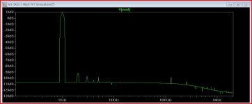
So I run the FFT plot. My version of spice gives 262144 as the default number of data points. That setting appears to alter the extent or bandwidth to which harmonics are displayed. So am I correct in assuming that a higher number isn't neccessarily better as most of what can be seen in the MHz and Ghz region will just be artifacts of simulation and have no bearing to reality ?
So that's the third question That's enough for now I think.
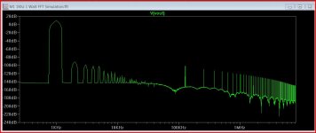
So here is the plot using a much reduced setting of 32768 and using the full extent of the data (0 to 8ms) and another using the more widely recommended 65536 points and a 4ms to 8ms time range. Although the result looks totally different the peaks are still at the same amplitudes.
Thanks for reading.
If anyone could contribute to this it would be much appreciated. I'm trying to keep this really simple and explain every step I take here.
So here we have the circuit set up for an output of 1 watt rms into 8 ohm. How would you set up a simulation to find a realsitic THD value for this ?
The settings I am using are these,
.op
.option noopiter (because the simulator can not find an operating point using the default method and the error log suggests adding this directive)
.option plotwinsize=0
.maxstep=0.488331106u I've read up on this and how to calculate the value (I think
) .four 1khz 10 4 v(vout) I understand that looks at the first 10 harmonics over the last four cycles.
.tran 8m
The input signal is 1khz for 16 cycles at a level that gives 1 watt rms output. So I run the simulation and get the following THD report showing 0.0011%.
So first question... is there any problem in the settings used so far to derive that figure ?
-----------------------------------------------------------------------------------------------------------------------------------------
Next part of the question...
The figures in the THD print out seem to be the figures that really matter. The FFT plot which I'll come to next can be made to look beter or worse depending on the settings used for the plot while keeping all the spice directives that were set above the same. To me, the text print out is the real guide here.
So second question. Is that a fair statement would you say ?
------------------------------------------------------------------------------------------------------------------------------------------
So I run the FFT plot. My version of spice gives 262144 as the default number of data points. That setting appears to alter the extent or bandwidth to which harmonics are displayed. So am I correct in assuming that a higher number isn't neccessarily better as most of what can be seen in the MHz and Ghz region will just be artifacts of simulation and have no bearing to reality ?
So that's the third question
That's enough for now I think.So here is the plot using a much reduced setting of 32768 and using the full extent of the data (0 to 8ms) and another using the more widely recommended 65536 points and a 4ms to 8ms time range. Although the result looks totally different the peaks are still at the same amplitudes.
Thanks for reading.
Attachments
Only use the .noopiter command if the simulation hangs while computing the operating point. It is normal for the first method to fail and SPICE to revert to Gmin stepping. In most cases the .noopiter command is not necessary and will not give a significant increase in performance.
Increased FFT samples will lower the noise floor and increase the frequency resolution. The biggest reason I found to use a large number was for a low noise floor. All this becomes trivial if you synch everything using my command set.
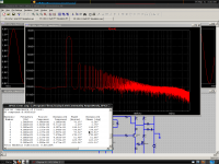
Your noise floor is wrong. It is flat line, this is not normal and it means potential is being wasted. First thing you need to do is to run the amp for at least 1 sine cycle before starting the simulation. This will get the drift and pulse caused by the abruptly starting sinewave input signal out of the measurement, and out of the FFT, greatly helping resolution. This is the only thing restricting your FFT, since you have no large time constants in the circuit.
It is best to give the simulator the equations, rather than numbers you calculated yourself, as the simulator has 32 bits of accuracy. This is why I use equations in my command set. Everything is nearly automatic, and trivial as long as you understand what the equations do.
First, I define the number of FFT samples I need:
.param FFT=2**16
Because the FFT sample number are selectable from powers of 2, it is easier just to change the exponent (the ** means a ^ to LTSpice). 2**16=65536. With everything synch'd you can get away with a much lower number of samples.
Next, I calculate the timestep for taking that many samples in the given simulator time frame.
.param timestep=10mS/FFT
Because I add an extra rev-up cycle to the beginning, I use this .tran command:
.tran 0 11m 1m {Timestep}
Your .four directive is messed up, it gives a 10-harmonic analysis by default so you only need this:
.four 1kHz v(vout)
Increased FFT samples will lower the noise floor and increase the frequency resolution. The biggest reason I found to use a large number was for a low noise floor. All this becomes trivial if you synch everything using my command set.
Your noise floor is wrong. It is flat line, this is not normal and it means potential is being wasted. First thing you need to do is to run the amp for at least 1 sine cycle before starting the simulation. This will get the drift and pulse caused by the abruptly starting sinewave input signal out of the measurement, and out of the FFT, greatly helping resolution. This is the only thing restricting your FFT, since you have no large time constants in the circuit.
It is best to give the simulator the equations, rather than numbers you calculated yourself, as the simulator has 32 bits of accuracy. This is why I use equations in my command set. Everything is nearly automatic, and trivial as long as you understand what the equations do.
First, I define the number of FFT samples I need:
.param FFT=2**16
Because the FFT sample number are selectable from powers of 2, it is easier just to change the exponent (the ** means a ^ to LTSpice). 2**16=65536. With everything synch'd you can get away with a much lower number of samples.
Next, I calculate the timestep for taking that many samples in the given simulator time frame.
.param timestep=10mS/FFT
Because I add an extra rev-up cycle to the beginning, I use this .tran command:
.tran 0 11m 1m {Timestep}
Your .four directive is messed up, it gives a 10-harmonic analysis by default so you only need this:
.four 1kHz v(vout)
Attachments
It is important to use a large number of samples because without a very low timestep/high samplerate, stability cannot be simulated correctly because the frequencies are beyond the Nyquist frequency.
Sleeping now! There is some more stuff in my command set that I can explain to you, it is a convenience really, there is not much more to it.
The noise floor can be decreased a little if you use more FFT samples than in your simulation, but it doesn't change much.
Sleeping now! There is some more stuff in my command set that I can explain to you, it is a convenience really, there is not much more to it.
The noise floor can be decreased a little if you use more FFT samples than in your simulation, but it doesn't change much.
Last edited:
Many thanks for taking the time to do that.
I'm going to have a play around to try and make more sense of it all now.
It's understanding the way it all fits together that is a steep learning curve. Such as the value {timestep} being entered in the CMD box for max timestep.
So that looks at and works the value out from the .param 10ms/FFT directive rather than working it all out manually.
I can tell when I run this how much longer the sim takes to run compared to my settings before.
Plenty to be going on with... many thanks.
To make the simulation faster, you can decrease 2**16 to 2**14 or something (but this falls prey to the caveat in post 23). Some fields require the {} braces to go around any variables or equations you enter, but the .param statements don't.
Those "twin tower" spikes from 100KHz onmward in your FFT are what happens when the simulation samples and FFT samples are not sync'd.
Finally, Cordell's models are good, but for BJTs they don't model quasi-saturation, so they will behave too well at very low Vce. No one models quasi-saturation really, so this is a major weak point in simulation.
If you want I can give you some sim files useful for verifying BJT curves with the datasheets. It is important look look at the Vcesat curves to see how simulation differs.
Thanks keantoken for all your help on this and the offer of the files.
Just getting a grasp of the basics is plenty to be going on with at the moment before I even think to start verifying models and so on.
The info you have given has been brilliant... and I want to make sure I understand it all before trying new things. Even things such as the parametric sweep function I haven't tried yet.
So a lot to learn
Glad to help. Having more experience with real circuits, you may soon teach me something about making simulations more realistic.
Now that is where it does get interesting, in seeing how real vs simulations compare.
Please post 'em!*snip*
If you want I can give you some sim files useful for verifying BJT curves with the datasheets. It is important look look at the Vcesat curves to see how simulation differs.
Wayne
Here they are. The biggest differences are usually found in the Vcesat/Hfe and Hfe graphs. Everything should be looked at in detail, for instance the KSC1845 model has cripplingly high Rc, which will ruin it's behavior in any current mirror; this is easily revealed by looking at the Vcesat curves.
I left the names from some of my experimental models in these files, if you run them as-is you will be told the model doesn't exist, so choose on of your own models to test out.
I left the names from some of my experimental models in these files, if you run them as-is you will be told the model doesn't exist, so choose on of your own models to test out.
Attachments
Having more experience with real circuits, you may soon teach me something about making simulations more realistic.
Now that is where it does get interesting, in seeing how real vs simulations compare.
Or, having listening to a lot of amps, we can simulate the amps that we have listened to and see how sounds correlate with simulations (also topologies).
Simple circuits and single ended circuits have typical FFT chart as it seems. I have simulated M1 (Mooly's amp) with SSA front end and the result is much "better" than the original M1. But I didn't build it because I have another "approach" for CFP output stage. Attached is 2 amps FFT simulations. None has been built (still working on it). The bipolar version of the first amp had been built and it sounded good even with much worse simulated distortion.
The first amp on the left has 60V rail. With 63V swing and 3R load it goes up to almost 1A per pair (2 pairs used). And with 59V swing the simulated distortion is not good enough. So I'm thinking about using front end regulator like Goldmund Mimesis3 or Os' CX amp. I still have to measure the transformers on hand first before deciding on the simulated rail voltage.
The second amp is my effort for CFP output with lowish (35V) rail. I believe it will sound better than the first amp, even tho the simulated distortions shows the opposite, because the topology is not compromised as the first one.
So, before comparing amps sounds with simulations, I think we have also to compare amps sounds with topologies. Well, I don't know, I'm a newbie myself
Attachments
Jay, you should really try to get the noise floor down. .four THD results will be totally wrong. Just adding a few rev-up cycles may help a lot.
The problem with comparing simulations and listening tests is that if you don't first make your simulation realistic, then the simulated amp won't behave like the one you're listening to. Running the simulator like a well-oiled machine contributes to much less sudden headaches, and less time fiddling with things other than the circuit.
The problem with comparing simulations and listening tests is that if you don't first make your simulation realistic, then the simulated amp won't behave like the one you're listening to. Running the simulator like a well-oiled machine contributes to much less sudden headaches, and less time fiddling with things other than the circuit.
Or, having listening to a lot of amps, we can simulate the amps that we have listened to and see how sounds correlate with simulations (also topologies).
Simple circuits and single ended circuits have typical FFT chart as it seems. I have simulated M1 (Mooly's amp) with SSA front end and the result is much "better" than the original M1. But I didn't build it because I have another "approach" for CFP output stage. Attached is 2 amps FFT simulations. None has been built (still working on it). The bipolar version of the first amp had been built and it sounded good even with much worse simulated distortion.
Here are two files, one for my amp and one for the now classic "Blameless Class B".
The Class B amp is one I built some years ago on the strength of it's performance figures alone. It was built correctly on the official PCB's with all components as specified at the time.
Subjectively the amp was typically "good HiFi", very clean, good control with a sort of "etched" quality to the music. It was the amp where a few selected recordings could sound really good, but many others did not. And that could be taken as the typical "well the amp is presenting it how it is "viewpoint".
And then I developed and built the M1. It was obvious on listening that this was very different, now pratically all recordings sounded not just good but absolutely compelling to listen to. There was no sense of fatigue and that false "etched" quality of the Blameless was gone.
It seems the reason why is down to the distribution of harmonics. Compare the relative amplitudes of the odds and evens between the two. Alter the amplitude of the input too. Set the blameless to give around 1 watt and compare.
There's no right and wrong answer to all this. If you wanted a lab amp that could be pushed to ever lower steady state figures then the M1 topology probably isn't the way to go. However, if you want an amp to really sing and be enjoyable to listen too then the Blameless topology does not seem to be the answer.
I always say that it doesn't matter how good your amp is on paper if you keep finding fault with it on listening to it, and then if you hear other amps that "sound" better then the amp your listening to isn't doing it's job an amplifier for music.
Also you have to remember that simulating like this is only half the story. You have to look at the amp with real signals and real loads.
In fact, this could be interesting...
Here is a derivative of the M1 using HEXFETS and real scope shots of the output into capacitive loads. How would LTSpice compare I wonder ?
http://www.diyaudio.com/forums/soli...-hexfet-poweramp-sonic-benefits-approach.html
Attachments
Jay, you should really try to get the noise floor down. .four THD results will be totally wrong. Just adding a few rev-up cycles may help a lot.
What do you mean by that (or why and how to be precise), Kean? The chart limits are manually edited so to compare both amps. But I believe you are referring more to the second one?
The problem with comparing simulations and listening tests is that if you don't first make your simulation realistic, then the simulated amp won't behave like the one you're listening to. Running the simulator like a well-oiled machine contributes to much less sudden headaches, and less time fiddling with things other than the circuit.
Yes, thanks, I'm sure you're right. I just don't know enough about amp design and simulation. But I can't wait those experts to design amps the way I want it so I have to start designing myself. And latfets, my favorite output devices, are expensive, so I started to design/build bipolar amps to ensure that I would be good enough when later I build my latfet amp

SSA in general is very wild. I believe real measurement is mandatory to get good result with the topology. The first amp simulation I posted was not SSA (but simple symmetrical). It is not wild. I can pick any transistors or use close value resistors and the result is not far away. The second one though, very sensitive to part changes.
In the past, people didn't use simulator. I use simulator mainly to help manual calculation (calculating the operating points).
Here are two files, one for my amp and one for the now classic "Blameless Class B".
The Class B amp is one I built some years ago on the strength of it's performance figures alone. It was built correctly on the official PCB's with all components as specified at the time.
Subjectively the amp was typically "good HiFi", very clean, good control with a sort of "etched" quality to the music. It was the amp where a few selected recordings could sound really good, but many others did not. And that could be taken as the typical "well the amp is presenting it how it is "viewpoint".
And then I developed and built the M1. It was obvious on listening that this was very different, now pratically all recordings sounded not just good but absolutely compelling to listen to. There was no sense of fatigue and that false "etched" quality of the Blameless was gone.
It seems the reason why is down to the distribution of harmonics. Compare the relative amplitudes of the odds and evens between the two. Alter the amplitude of the input too. Set the blameless to give around 1 watt and compare.
There's no right and wrong answer to all this. If you wanted a lab amp that could be pushed to ever lower steady state figures then the M1 topology probably isn't the way to go. However, if you want an amp to really sing and be enjoyable to listen too then the Blameless topology does not seem to be the answer.
I always say that it doesn't matter how good your amp is on paper if you keep finding fault with it on listening to it, and then if you hear other amps that "sound" better then the amp your listening to isn't doing it's job an amplifier for music.
Also you have to remember that simulating like this is only half the story. You have to look at the amp with real signals and real loads.
In fact, this could be interesting...
Here is a derivative of the M1 using HEXFETS and real scope shots of the output into capacitive loads. How would LTSpice compare I wonder ?
http://www.diyaudio.com/forums/soli...-hexfet-poweramp-sonic-benefits-approach.html
Yes, I'm agree with you (I have built both your amp and the Blameless). And I think "topology" is more important, at least to me. By topology I mean something in the circuit that you can see by eyes, a feature to increase stability or to achieve certain objective but has drawback as a compensation.
Blameless for example, is I think one of a few modern amp where the output of the driver is not connected to the output, nor to ground. This is becoming a "standard" for good sounding amps imo. The 100pF compensation cap in the VAS is just too big. If the amp requires it, then the amp doesn't deserve a build. The input LTP is not my favorite either.
Here is a derivative of the M1 using HEXFETS and real scope shots of the output into capacitive loads. How would LTSpice compare I wonder ?
http://www.diyaudio.com/forums/soli...-hexfet-poweramp-sonic-benefits-approach.html
Wow, how can I missed that 2008 thread??? Thanks, it will be an interesting read, simulation and building
Wow, how can I missed that 2008 thread??? Thanks, it will be an interesting read, simulation and building
Here's a simulation of that amp. This takes a minute or so to run due to needing a longer simulation run over 110ms.
Notice the far higher (to be expected) distortion and its spectrum.
This would be interesting to do with with laterals but would need multiple pairs to overcome the low transconductance.
Attachments
- Status
- This old topic is closed. If you want to reopen this topic, contact a moderator using the "Report Post" button.
- Home
- Design & Build
- Software Tools
- LTSpice FFT simulation settings and inconsistent results.