I've been using LTSpice for a couple of years now, and recently started playing around with the FFT analysis. I confess to being rather confused with the results I'm getting. Perhaps I should say at this point that I don't consider a Spice analysis to be a substitute for the real thing. I realize that a simulation is only as good as the tube models used, that simulation doesn't reflect real world variances between nominally identical devices and that, in consequence, an FFT cannot predict exactly what the end product will sound like, if it ever gets built.
The LTSpice FFT function requires me to select the number of points used in the analysis, so I've started experimenting with this, to see its effect. I've found that the more points included in the FFT analysis , the smoother the graph becomes, the lower the harmonic distortion and the fewer harmonics are present. At one extreme (low number of points analyzed e.g. 13), I get significant harmonic distortion, including 3rd, 5th, 7th, 9th and 11th harmonics. At the other extreme (large number of points analyzed e.g. 61) I get virtually no distortion, with only 3rd and a tiny bit of 5th. I have no idea which of these results is more correct or if the 'truth' lies somewhere in between. This is a P-P amp, so there is no even-order harmonic distortion.
Like many aspects of LTSpice, the FFT analysis is not explained in 'help', so there is no guidance on how to get the most meaningful result. Also, I can't find anything relevant at the Yahoo Groups LTSpice users' forum, so I thought I should ask for advice here: does anyone know what would be a sensible number of points to include?
I'm haven't used the FFT in LTSpice yet, but one thing that likely is required is to start and end the data set on the same similar phase point of the test sinewave accurately. (More accurately, the next data point, following your last data point, should be the same as your 1st data point, for a repetitive sinewave signal.) The FFT math assumes the data set repeats endlessly, so any misalignment here will cause weird artifacts in the spectrum.
The sampling theorem would indicate a minimum of 2 data points to capture the fundamental test harmonic and N times as many points to get the Nth harmonic. Practically speaking, I would use more like 8 times that many points or more.
Many FFT algorithms also require 2 to some M power points for efficient calculation, so often one will see something like 1024 or 4096 data points used. This in turn can lead one to use a 1.024 KHz test signal, so it comes out accurately repeating in say 1024, 1 usec. spaced, data points.
Good luck,
Don
remember to add:
.option plotwinsize=0
to turn off data compression
lots of points, both fine time step in .tran and fft points are good ideas, I default at 131K points, Blackman window - always needs 4X the fundamental period analysis time but minimizes spectal splatter
many pointers throughout my posts, search
user: jcx
keywords: fft ltspice
show posts
"I default at 131K points, Blackman window - always needs 4X the fundamental period analysis time but minimizes spectal splatter"
Ah, so LTSpice has FFT windowing functions available.
This eliminates the need for a binary number of data points and long steady state settling time, but requires 4 times as many data points. The data are windowed, time wise, by a Gaussian or similar ramp up - ramp down type function. So that imperfect matching of the beginning data with the ending data (maybe some DC transient still occuring in the data say) is minimized. Requires lots of processing power though, so helps to have a 1 GHz or faster CPU.
Don
Hi Ray. Here are a couple more suggestions to help generate clean FFT plots. Turning off data compression has already been mentioned. It's crucial, as is ensuring the simulation time (or the selected time window for FFT) capture a waveform starting and ending at zero crossings.
In the FFT menu is a parameter window labeled "Number of data point samples in time". I usually set it to 65536. In the schematic half under "Edit Simulation Command" > Transient, set Timeslice to the reciprocal of the number of data point samples selected for FFT, in this case 1/65536 or 0.0000152587890625. I'm not familiar with the relative benefits of different windowing functions but have been told by pros in the field that Blackman is the way to go so typically leave it at that.
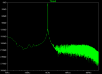
One caveat. LTSpice appears to have an oddity regarding data caching. Sometimes making these changes mid-session results in unusual FFT plots, for example large spikes above 100 kHz. Closing and restarting the session always clears it. As a sanity check I set the signal source as ideal - no output impedance or parasitics - and run an FFT on it to insure it's 'perfect'. When correct it looks like graph below.
In the FFT menu is a parameter window labeled "Number of data point samples in time". I usually set it to 65536. In the schematic half under "Edit Simulation Command" > Transient, set Timeslice to the reciprocal of the number of data point samples selected for FFT, in this case 1/65536 or 0.0000152587890625. I'm not familiar with the relative benefits of different windowing functions but have been told by pros in the field that Blackman is the way to go so typically leave it at that.
One caveat. LTSpice appears to have an oddity regarding data caching. Sometimes making these changes mid-session results in unusual FFT plots, for example large spikes above 100 kHz. Closing and restarting the session always clears it. As a sanity check I set the signal source as ideal - no output impedance or parasitics - and run an FFT on it to insure it's 'perfect'. When correct it looks like graph below.
Attachments
Thanks for the helpful suggestions. I've never tried the Blackman window, but I will.
What I have been trying is to run the transient analysis for 30 seconds, with an input signal of 1kHz starting after a delay varying from 29.6 to 29.8 seconds. I then zoom in to show the output trace only for the period that the signal is on. I run the FFT analysis for the same period as the signal ('Use current zoom extent'). There is a big difference in results depending on the signal delay.
I've also tried using different values (number of points) for the binomial smoothing and found that I get cleaner-looking results if I make this number much bigger than the default of 5 (around 45 or more).
Thirty seconds? I envy anyone with a personal Cray. ")
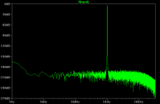
Long runs before data capture begins allow 'the circuit' to stabilize. Not all require it. The graphs posted earlier - a simple LED biased, choke loaded, R-coupled two 12at7 circuit - was based on a 200 msec total run, from 0-100 msec for warmup and data captured from 100 to 200 msec with a 1000 Hz source. Obviously, that works out to 100 full cycles at 1000 Hz (but only 10 at 100 Hz.)
As another sanity check the same sim as above was run under identical conditions except 1 sec was added to both parameters. Capture began at 1100 msec and ended at 1200 msec. In this case 100 msec of warmup is apparently plenty for computational accuracy well exceeding that of the tube model, the distrotion harmonics were unaffected.
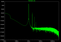
Long capture periods are great for improving resolution and low frequency accuracy, though it's a judgement call if the additional information is useful. The sim above was altered to capture a full second of data after the same 1100 msec of warm up. The input spectrum is shown below.
Long runs before data capture begins allow 'the circuit' to stabilize. Not all require it. The graphs posted earlier - a simple LED biased, choke loaded, R-coupled two 12at7 circuit - was based on a 200 msec total run, from 0-100 msec for warmup and data captured from 100 to 200 msec with a 1000 Hz source. Obviously, that works out to 100 full cycles at 1000 Hz (but only 10 at 100 Hz.)
As another sanity check the same sim as above was run under identical conditions except 1 sec was added to both parameters. Capture began at 1100 msec and ended at 1200 msec. In this case 100 msec of warmup is apparently plenty for computational accuracy well exceeding that of the tube model, the distrotion harmonics were unaffected.
Long capture periods are great for improving resolution and low frequency accuracy, though it's a judgement call if the additional information is useful. The sim above was altered to capture a full second of data after the same 1100 msec of warm up. The input spectrum is shown below.
Attachments
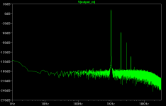
And the output here. Certainly the skirts are much tighter and the low frequency accuracy greatly improved. It's questionable if the added computational time gains any useful information, the harmonics haven't changed noticably.
Also, sorry for not being clear earlier. I run the FFT on the full captured waveform: "Use Extent of Simulation Data". The FFT period is in effect fully set by the .tran directive.
Also, sorry for not being clear earlier. I run the FFT on the full captured waveform: "Use Extent of Simulation Data". The FFT period is in effect fully set by the .tran directive.
Attachments
LTSpice Harmonic Analysis
I am also new to LTSpice, and I've also noticed the different results obtained according to different Time settings (time simulation and length of time steps).
But after many experiments and trials I concluded that the simulation time must be long and the simulation time steps small.
The length of simulation time and the related length of time step can be found doing simulation time incremental and time step decremental repetitive trials.
In each trial I increment the simulation time length and simultaneously I decrement the length of time step. After few trials, further incrementation of simulation time and decrementation of time step does not affect the harmonic analysis results anymore.
In other words the results are "stabilized" not affected by further simulation time increments and time step decrements.
The combination of the minimum simulation time and the corresponding maximum time step, where the harmonic results become constant ("stabilized") are the required time settings.
If someone does it once for a special frequency, say 1000 Hz, then he can keep in mind these settings and he can reuse them in future experiments for the same circuit and the same frequency.
These settings are also "valid" for harmonic simulations of frequencies near the initial frequency (say of the same order, but not take it literally). For example the settings for simulating 1000Hz can be the same for simulating 2000Hz.
In other words, I think that the correct results are exactly these constant (stabilized) results.
I also think that repetitive computing procedures, depending on variable data (time), have similar behavior.
By the way, does anyone know where can I find LTSpice models for BC184, BC214, BC516, BC517? I will appreciate any help!!!.
- Status
- This old topic is closed. If you want to reopen this topic, contact a moderator using the "Report Post" button.
- Home
- Design & Build
- Software Tools
- How to make sense of LTSpice FFT analysis?