I don't use any Green function. The simulated acoustic radiation is a brute force approach based on Huygens-Fresnel decomposition of sources and real-time superposition of all radiations at listener place.
I looked up Huygens-Fresnel in Wiki and it appears that these are based on a Greens function. That's what the propagation function is.
Why not do it here ?
Personally, I'd like the OP to confirm that. It's his tread and I liked what he was doing.
POST #7
C. Infinite Line Source: frequency-domain pressure response
Coordinates : Imagine, if you will, a rather standard 3-D (rectangular) coordinate system, comprised of the 3 classic, orthogonal axes : x, y and z") We'll consider the x-y plane being the "horizontal" plane, with the z-axis extending "vertically".
We'll consider the x-y plane being the "horizontal" plane, with the z-axis extending "vertically".
We're going to build our Infinite Line Source along (coincident with) the vertical z-axis The Infinite Line Source will have a constant volume acceleration per-unit-length of "Al".
But we start with baby steps Here's how we proceed :
First, let's consider a little (VERY little) "piece" of the Infinite Line Source, at some point "z" along the z-axis (meaning, our little "piece" will be at a distance "z" from the origin). Our little "piece" of the Infinite Line Source has a small (VERY small) length of "dz".
Now the clever bit : our little (VERY little) piece behaves just like an elemental monopole point-source ... which we just analyzed ... radiating with constant volume acceleration of (Al*dz)
What we need, to complete our fist step, is to identify the pressure measured at some random point in space, resulting from our little piece/elemental monopole. Let's start by placing our measuring point on the specific x-y plane of z=0, at a radial distance of "r" from the z-axis. The symmetry of our arrangement dictates that all measuring points at a distance of "r" from the z-axis will receive the same pressure from our little piece, no matter where in the x-y plane those measuring points reside. We also know that our little piece of the line is acting like an elemental monopole at some vertical height of "z". What's the distance from the little piece to our measuring point? Let's call it "R" ... Pythagoras reveals the result for us :
R^2 = r^2 + z^2
R = sqrt[r^2 + z^2]
Now we have what we need, to write the pressure from our little piece (VERY little) ... where the little piece is at some point "z" along the line, and we are measuring at some radial distance "r" from the line, in the x-y plane of z=0 We'll simply recall the pressure we discussed from a point-source, to identify :
pressure at "r" from little piece of line = {Al*dz} * {exp[jwt]} * {[rho/(4pi*R)] * exp[-jkR]}
where k = wavenumber = w/c
w= frequency
c = speed of sound
(we'll soon be ignoring that exp[jwt] term, because it's the time-dependent excitation ... which i like to separate from my "transfer function" analysis)
next up : we'll add-up all of our little pieces, to form the infinitely long line
C. Infinite Line Source: frequency-domain pressure response
Coordinates : Imagine, if you will, a rather standard 3-D (rectangular) coordinate system, comprised of the 3 classic, orthogonal axes : x, y and z
We'll consider the x-y plane being the "horizontal" plane, with the z-axis extending "vertically".We're going to build our Infinite Line Source along (coincident with) the vertical z-axis
The Infinite Line Source will have a constant volume acceleration per-unit-length of "Al".But we start with baby steps
Here's how we proceed :First, let's consider a little (VERY little) "piece" of the Infinite Line Source, at some point "z" along the z-axis (meaning, our little "piece" will be at a distance "z" from the origin). Our little "piece" of the Infinite Line Source has a small (VERY small) length of "dz".
Now the clever bit : our little (VERY little) piece behaves just like an elemental monopole point-source ... which we just analyzed ... radiating with constant volume acceleration of (Al*dz)
What we need, to complete our fist step, is to identify the pressure measured at some random point in space, resulting from our little piece/elemental monopole. Let's start by placing our measuring point on the specific x-y plane of z=0, at a radial distance of "r" from the z-axis. The symmetry of our arrangement dictates that all measuring points at a distance of "r" from the z-axis will receive the same pressure from our little piece, no matter where in the x-y plane those measuring points reside. We also know that our little piece of the line is acting like an elemental monopole at some vertical height of "z". What's the distance from the little piece to our measuring point? Let's call it "R" ... Pythagoras reveals the result for us :
R^2 = r^2 + z^2
R = sqrt[r^2 + z^2]
Now we have what we need, to write the pressure from our little piece (VERY little) ... where the little piece is at some point "z" along the line, and we are measuring at some radial distance "r" from the line, in the x-y plane of z=0
We'll simply recall the pressure we discussed from a point-source, to identify :pressure at "r" from little piece of line = {Al*dz} * {exp[jwt]} * {[rho/(4pi*R)] * exp[-jkR]}
where k = wavenumber = w/c
w= frequency
c = speed of sound
(we'll soon be ignoring that exp[jwt] term, because it's the time-dependent excitation ... which i like to separate from my "transfer function" analysis)
next up : we'll add-up all of our little pieces, to form the infinitely long line
I looked up Huygens-Fresnel in Wiki and it appears that these are based on a Greens function. That's what the propagation function is.
Personally, I'd like the OP to confirm that. It's his tread and I liked what he was doing.
Gentlemen, thank you for the respect
please feel free to take this thread in any direction at all, i rather like the engagement ... including detours I'm labeling the main direction with "post numbers", so that readers can stay on the main street easily, if they so choose
Green's functions are solutions to wav equation in case of Huygens-Fresnel sources, but I don't need to use Green's functions.I looked up Huygens-Fresnel in Wiki and it appears that these are based on a Greens function. That's what the propagation function is.
I will try to explain the bases : look at post #7 just above and consider just one tiny point source. Signal at listener place is same as source signal but delayed and attenuated depending on this source to listener distance.
Consider another tiny point source : signal at listener is same as this source signal but delayed and attenuated depending on this distance.
Now total signal at listener due to those two sources is simply the real time addition of both signals.
For many sources, just add all signals : divide each loudspeaker in many tiny point sources. And a line array is just many loudspeakers.
Now computers are fast enough to process thousands of signals in real time.
With this brute force approach, you don't need to solve any equation.
It's quite simple but I have not seen this method used before.
Last edited:
Whether or not you realize it you are using exactly the Green's Function approach to find the attenuation and the delay of each element, and the functions that you are using are the free field ones, hence you are not accounting for many aspects of the problem like diffraction of the enclosure, etc. Its an interesting approach to "real time" analysis, but people have been doing this off-line for more than a century. I am not sure that the limit on accuracy required to do real-time is a major advantage to a more accurate model that just takes a few more minutes. BEM and FEA, for example, can do this problem to an extremely high accuracy, just not in real time.
For attenuation and delay, I just have to calculate the distance. Diffraction of the enclosure is simulated by many secondary sources. Reflections (walls, floor,...) are simulated by image sources. It is just a question of accuracy vs computing power.Whether or not you realize it you are using exactly the Green's Function approach to find the attenuation and the delay of each element, and the functions that you are using are the free field ones, hence you are not accounting for many aspects of the problem like diffraction of the enclosure, etc. Its an interesting approach to "real time" analysis, but people have been doing this off-line for more than a century. I am not sure that the limit on accuracy required to do real-time is a major advantage to a more accurate model that just takes a few more minutes. BEM and FEA, for example, can do this problem to an extremely high accuracy, just not in real time.
Also, for accuracy of primary sources and diffraction sources, you may not allways use point sources : an obliquity factor (see Kirchhof's diffraction) should sometimes be used.
One advantage is a true real time auralization (not a convolution) : you can change a parameter or a position while listening to the result.
Last edited:
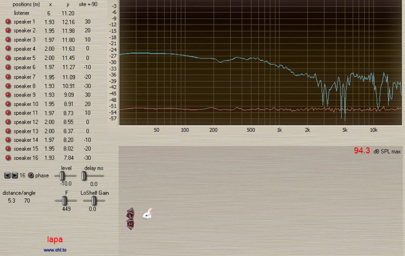
To explain the method, I just published a (basic) video here :
lapa - YouTube
lapa - YouTube
Last edited:
Looks like a nice piece of software. Why does the screen change for every type of analysis? Does each analysis have to be compiled or do the variables automatically show up as sliders?
I have never been much in favor of auralization except in the case of research, because in valid tests of "sound quality" they must be done blind. However a researcher could setup very nice tests with your software, which I would love to do. The only thing is that we have no money at all for this kind of testing - I typically do all the simulations myself and Lidia just uses her lab. Funding is never available. How would you like to donate this software for studies of diffraction, etc?
I have never been much in favor of auralization except in the case of research, because in valid tests of "sound quality" they must be done blind. However a researcher could setup very nice tests with your software, which I would love to do. The only thing is that we have no money at all for this kind of testing - I typically do all the simulations myself and Lidia just uses her lab. Funding is never available. How would you like to donate this software for studies of diffraction, etc?
My basic question was : what phenomenas (distortions) are audible and to which level ? And to understand, you need to separate variables.
So I did one software to listen to diffraction, one for crossover auralization, one for reflexions and room modes, one for arrays, one for cardioid loudspeakers in a room, etc....
At the end, I could mix everything into one software only. The main problem would be too many parameters to set.
One tricky simulation is the waveguide (Earl knows it well), I tried to simulate it with image sources but it quickly gets very complicated.
To Earl : for research purposes, I would be glad to give you any software (for free of course).
Last edited:
And what about the head diffraction? Do you have any, a generic model or does it allow for specific HRTFs to be used?
The reason that I ask is that Lidia and I are currently doing some research on very early wall reflections. We could certainly use software like that to generate our test signals. You could generate them and we would credit the software in our paper. That could be a big boost to your marketing. E-mail me directly at egeddes@gedlee.com if this interests you.
The reason that I ask is that Lidia and I are currently doing some research on very early wall reflections. We could certainly use software like that to generate our test signals. You could generate them and we would credit the software in our paper. That could be a big boost to your marketing. E-mail me directly at egeddes@gedlee.com if this interests you.
Last edited:
Please send me the position (ie x,y,z at voice coil) of each driver in metric values and exact angle (it seems to be less than 15°), so I can do the simulation.Design #1 uses 8 P7's per side. Each driver in a sealed rectangular MDF enclosure 5/8"(.016m) thick.
Internal measurements on this common enclosure is 9 1/4"(.235m) length, 4 1/2"(.114m) height and 4 1/2" width. Very minimal internal stuffing.
Here is the best pic I have of this setup. Please ignore the tweeter in the middle. I estimate the angle about 15degrees between each enclosure.
I have no way to measure the angles. For Design 1 with the 8x rectangular enclosures, that I spec'd in the earlier post, I'll have to approximate the measurements because they've been disassembled already.
X=0 for all since drivers are aligned vertically.
..* Z=-7.62cm, Y=215.90cm
...* Z=-5.08cm, Y=198.12cm
....* Z=-2.54cm, Y=180.34cm
.....* Z=0, Y=162.56cm
.....* Z=0, Y=144.78cm
....* Z=-2.54cm, Y=127cm
...* Z=-5.08cm, Y=109.22cm
..* Z=-7.62cm, Y=91.44cm
I would approximate the angles at 10/15? degrees, except the middle 2 drivers. Those 2 are level with the floor.
jlo, thanks for taking the time to do this!
Last edited:
POST #8
C. Infinite Line Source: frequency-domain pressure response (continued)
In the last post, we identified the pressure anywhere on the x-y plane (at z=0), at some distance "r" from z-axis, resulting from any little elemental monopole located at some point "z" along the z-axis:
{Al*dz}*{exp[jwt]}*{[rho/(4pi*R)]*exp[-jkR]}
where
R = sqrt[r^2 + z^2]
Perhaps this is obvious ... but we took this small step first, because we can consider an Infinite Line Source to be made up of an infinite series of these elemental monopoles along the z-axis
Before we take our next step, please note that pressure is a scalar quantity. This means that we can ultimately find the measured pressure (at that same point on the x-y plane, some distance "r" from the z-axis) from our newly-constructed Infinite Line Source by simply adding the pressure from all of the tiny little monopoles that make-up our infinite line
Since we're adding an infinite number of tiny little things, we'll call it integration and immediately write:
p(r,t) = INT[Al*exp[jwt]*[rho/(4pi*R)]*exp[-jkR]]dz, from z = -infinity to +infinity
Now we'll take a few things out of the integral that don't depend on the integration variable "z", and ignore the Al*exp[jwt] term that i've associated with the "source", in order to write down what i'll call the pressure transfer function from the Infinite Line Source:
p(r) = (rho/4pi)*INT[(1/R)*exp[-jkR]]dz, from z = -infinity to +infinity
p(r) = (rho/2pi)*INT[(1/R)*exp[-jkR]]dz, from z = zero to infinity
In somewhat more familiar "transfer function" lingo (written as a function of frequency),
H(k) = (rho/2pi)*INT[(1/R)*exp[-jkR]]dz, from z = zero to infinity
where
R = sqrt[r^2 + z^2]
k = wavenumber = w/c
A few notes, before we "solve" this integral :
1. Note that the resulting pressure will only depend on "k" and "r", because "z" is the integration variable (which will disappear in the result).
2. Note also that, once we "solve" the integral for any point on the x-y plane at z=0 (at some distance "r" from the z-axis), the infinite nature of the line source tells us that the result will be valid for ANY point on ANY x-y plane, at some radial distance "r" from the line source. In short, the result will NOT depend on height (as expected, for an infinite line source).
3. Whenever you add an infinite number of things, it's quite possible for the result to be "unbounded" fortunately, in this case, the result is "bounded" (as long as kr>0 )
C. Infinite Line Source: frequency-domain pressure response (continued)
In the last post, we identified the pressure anywhere on the x-y plane (at z=0), at some distance "r" from z-axis, resulting from any little elemental monopole located at some point "z" along the z-axis:
{Al*dz}*{exp[jwt]}*{[rho/(4pi*R)]*exp[-jkR]}
where
R = sqrt[r^2 + z^2]
Perhaps this is obvious ... but we took this small step first, because we can consider an Infinite Line Source to be made up of an infinite series of these elemental monopoles along the z-axis
Before we take our next step, please note that pressure is a scalar quantity. This means that we can ultimately find the measured pressure (at that same point on the x-y plane, some distance "r" from the z-axis) from our newly-constructed Infinite Line Source by simply adding the pressure from all of the tiny little monopoles that make-up our infinite line
Since we're adding an infinite number of tiny little things, we'll call it integration
and immediately write:p(r,t) = INT[Al*exp[jwt]*[rho/(4pi*R)]*exp[-jkR]]dz, from z = -infinity to +infinity
Now we'll take a few things out of the integral that don't depend on the integration variable "z", and ignore the Al*exp[jwt] term that i've associated with the "source", in order to write down what i'll call the pressure transfer function from the Infinite Line Source:
p(r) = (rho/4pi)*INT[(1/R)*exp[-jkR]]dz, from z = -infinity to +infinity
p(r) = (rho/2pi)*INT[(1/R)*exp[-jkR]]dz, from z = zero to infinity
In somewhat more familiar "transfer function" lingo (written as a function of frequency),
H(k) = (rho/2pi)*INT[(1/R)*exp[-jkR]]dz, from z = zero to infinity
where
R = sqrt[r^2 + z^2]
k = wavenumber = w/c
A few notes, before we "solve"
this integral :1. Note that the resulting pressure will only depend on "k" and "r", because "z" is the integration variable (which will disappear in the result).
2. Note also that, once we "solve" the integral for any point on the x-y plane at z=0 (at some distance "r" from the z-axis), the infinite nature of the line source tells us that the result will be valid for ANY point on ANY x-y plane, at some radial distance "r" from the line source. In short, the result will NOT depend on height (as expected, for an infinite line source).
3. Whenever you add an infinite number of things, it's quite possible for the result to be "unbounded"
fortunately, in this case, the result is "bounded" (as long as kr>0 ) Looks like a nice piece of software.
A researcher could setup very nice tests with your software, which I would love to do. How would you like to donate this software for studies of diffraction, etc?
I wanted to publicly thank Jean-Luc for his generous support of our research. He has graciously lent us his software, tailored to our needs, which saved us (me!) a tremendous amount of time. His help and support are most appreciated.
Hi Dr1v3n, I did a first simulation with your 8 loudspeakers alone or with floor reflection (no reflection attenuation or 10dB attenuation).I have no way to measure the angles. For Design 1 with the 8x rectangular enclosures, that I spec'd in the earlier post, I'll have to approximate the measurements because they've been disassembled already.
I would approximate the angles at 10/15? degrees, except the middle 2 drivers. Those 2 are level with the floor.
jlo, thanks for taking the time to do this!
See pictures with varying listener position at height 1.2m and distance varying from 3m to 6m
difficult to read ! (sorry first picture was wrong at height)
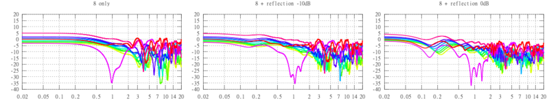
here with listener at 3m (all heights are relative to a simulated floor at 10m height, the simulated floor creates 8 new loudspeakers as image-sources)
Last edited:
JL, thank your sir! No rush at all, take your time. And thanks to werewolf for tolerating tangients to this array thread.
Everything above 200Hz follows a similar pattern I've seen while using REW and UMIC 1 mic. i.e. more SPL on bass and gentle slope down towards 20kHz.
Looks like HF reflections are killing a better FR. BUT no serious lobing effects, which I noticed did disappear for myself after 'curving' both arrays at listening distance 3'-4' away.
Will post more exact XYZ for Design 2 soon.
POST #9
C. Infinite Line Source: frequency-domain pressure response (continued)
In the last post, we found the frequency-domain "transfer function" from our Infinite Line Source to be :
H(k) = (rho/2pi)*INT[(1/R)*exp[-jkR]]dz, from z = zero to +infinity
where
R = sqrt[r^2 + z^2]
k = wavenumber = w/c
Our job now, is to work on this integral So let's change variables! (my bag of tricks to "solve" integrals isn't particularly deep, but changing variables is certainly among the classics)
Let:
z = r*sinh[v] (where sinh[v] is the hyperbolic sine function)
so that :
dz/dv = r*cosh[v] (where cosh[v] is the hyperbolic cosine function)
and :
R^2 = r^2 + z^2 = r^2*{1 + sinh^2[v]} = r^2*cosh^2[v]
or
R = r*cosh[v]
Our integral becomes :
H(k) = (rho/2pi)*INT[exp[-jkr*cosh[v]]]dv, from v=0 to +infinity
which can be separated into real & imaginary parts, eliminating the complex exponential:
H(k) = (rho/2pi)*{INT[cos[kr*cosh[v]]]dv - j*INT[sin[kr*cosh[v]]]dv}, from v=0 to +infinity (for both integrals)
What have we done !? Taking sines and cosines of the hyperbolic cosine function inside of integrals doesn't necessarily seem to make things easier but stay tuned ...
C. Infinite Line Source: frequency-domain pressure response (continued)
In the last post, we found the frequency-domain "transfer function" from our Infinite Line Source to be :
H(k) = (rho/2pi)*INT[(1/R)*exp[-jkR]]dz, from z = zero to +infinity
where
R = sqrt[r^2 + z^2]
k = wavenumber = w/c
Our job now, is to work on this integral
So let's change variables! (my bag of tricks to "solve" integrals isn't particularly deep, but changing variables is certainly among the classics)Let:
z = r*sinh[v] (where sinh[v] is the hyperbolic sine function)
so that :
dz/dv = r*cosh[v] (where cosh[v] is the hyperbolic cosine function)
and :
R^2 = r^2 + z^2 = r^2*{1 + sinh^2[v]} = r^2*cosh^2[v]
or
R = r*cosh[v]
Our integral becomes :
H(k) = (rho/2pi)*INT[exp[-jkr*cosh[v]]]dv, from v=0 to +infinity
which can be separated into real & imaginary parts, eliminating the complex exponential:
H(k) = (rho/2pi)*{INT[cos[kr*cosh[v]]]dv - j*INT[sin[kr*cosh[v]]]dv}, from v=0 to +infinity (for both integrals)
What have we done !? Taking sines and cosines of the hyperbolic cosine function inside of integrals doesn't necessarily seem to make things easier
but stay tuned ...- Status
- This old topic is closed. If you want to reopen this topic, contact a moderator using the "Report Post" button.
- Home
- Loudspeakers
- Multi-Way
- Infinite Line Source: analysis