How heavy compared to the solution within the working section? Although costly a typical PML implementation (there are different ones) should use something like 10% or so computational resources compared to the working section and so not make much difference to what is required for a full simulation. I presume you have seen a cost much larger than this that has prompted a switch to a substantially worse exit boundary condition?I'm using the second order SBC as described here: https://www.comsol.com/blogs/using-...onditions-for-wave-electromagnetics-problems/
Initially I used the PML, but that was too computationally heavy for the HF area.
Thanks!Impressive work!
For the low frequencies I agree, but as I'm approaching 20 kHz it's at least 100 % increase. And as most of the sim time is used above 10 kHz it really affects the total solution time. This is however not the main problem, I'm having some convergence issues with the PML for unknown reasons.How heavy compared to the solution within the working section? Although costly a typical PML implementation (there are different ones) should use something like 10% or so computational resources compared to the working section and so not make much difference to what is required for a full simulation. I presume you have seen a cost much larger than this that has prompted a switch to a substantially worse exit boundary condition?
/Anton
This seems to be the wrong way round. At high frequencies a PML that is, say, 5 cells deep will be a small proportion of the large number of small cells in the working section. At low frequencies when the cells in the working section are larger a 5 cell deep PML will be a larger proportion of the total number of cells.For the low frequencies I agree, but as I'm approaching 20 kHz it's at least 100 % increase. And as most of the sim time is used above 10 kHz it really affects the total solution time.
To sort that one out you are likely to need someone familiar with the particular PML implementation. A question for COMSOL support.This is however not the main problem, I'm having some convergence issues with the PML for unknown reasons.
For a fix geometry I agree. My geometry decreases with increasing frequency though. I'll do a little more research on how to set up the PML, but I feel like a second order SBC should be fine.This seems to be the wrong way round. At high frequencies a PML that is, say, 5 cells deep will be a small proportion of the large number of small cells in the working section. At low frequencies when the cells in the working section are larger a 5 cell deep PML will be a larger proportion of the total number of cells.
To sort that one out you are likely to need someone familiar with the particular PML implementation. A question for COMSOL support.
Right now I'm doing a comparison on elements/wavelength to see that the amount that I've chosen (6) is enough. Then I'm moving on to sim the waveguide in box (instead of infinite baffle).
/Anton
Comparison with denser mesh
I ran the sim for the proposed superelliptical waveguide with varying amount of elements/wavelength (5, 6, 7) to see if the mesh was dense enough. COMSOL recommends to use at least 5 elements. I have a mesh that is twice as dense on the membrane and thrice as dense on the mouth edge.
Results
Horisontal (on tweeter level):

Horisontal (3 dm above/below tweeter level):

The differences are subtle and only visible below 4 kHz.
The sim time was:
5 elements/wavelength: 5 minutes
6 elements/wavelength: 9 minutes
7 elements/wavelength: 16 minutes
Conclusion: 6 elements/wavelength seems ok. Increasing the accuracy of simulations should be done with other means than increasing mesh density.
/Anton
I ran the sim for the proposed superelliptical waveguide with varying amount of elements/wavelength (5, 6, 7) to see if the mesh was dense enough. COMSOL recommends to use at least 5 elements. I have a mesh that is twice as dense on the membrane and thrice as dense on the mouth edge.
Results
Horisontal (on tweeter level):
Horisontal (3 dm above/below tweeter level):
The differences are subtle and only visible below 4 kHz.
The sim time was:
5 elements/wavelength: 5 minutes
6 elements/wavelength: 9 minutes
7 elements/wavelength: 16 minutes
Conclusion: 6 elements/wavelength seems ok. Increasing the accuracy of simulations should be done with other means than increasing mesh density.
/Anton
You need to change the spacing by a significant amount which is normally a doubling or halving. The differences should show up at high frequencies not low frequencies. What is causing differences at low frequencies? Why are differences not being seen at high frequencies?Conclusion: 6 elements/wavelength seems ok. Increasing the accuracy of simulations should be done with other means than increasing mesh density.
In a study like this you need to be able to see the what you are measuring. I would suggest running 2, 4, 8, 16, 32 elements per wavelength on a 2D grid and plotting something sensitive to numerical error. If the grid is created by subdivision then something that usually works well is to take the solution with the 32 elements per wavelength as a reference, evaluate the error norm for the other solutions with respect to the reference and plot on a log axis. The slope of the error reduction should follow the order of the numerical scheme. If it doesn't then some other error is swamping the discretisation error (or the numerical scheme is inconsistent which is unlikely for an established commercial code). That some other error is likely to be a incorrect or misbehaving boundary condition.
This reply is majoring on the ability to check the results.You need to change the spacing by a significant amount which is normally a doubling or halving. The differences should show up at high frequencies not low frequencies. What is causing differences at low frequencies? Why are differences not being seen at high frequencies?
In a study like this you need to be able to see the what you are measuring. I would suggest running 2, 4, 8, 16, 32 elements per wavelength on a 2D grid and plotting something sensitive to numerical error. If the grid is created by subdivision then something that usually works well is to take the solution with the 32 elements per wavelength as a reference, evaluate the error norm for the other solutions with respect to the reference and plot on a log axis. The slope of the error reduction should follow the order of the numerical scheme. If it doesn't then some other error is swamping the discretisation error (or the numerical scheme is inconsistent which is unlikely for an established commercial code). That some other error is likely to be a incorrect or misbehaving boundary condition.
One must be able to ask the questions (the way you enter data into the simulator software) in such a way that one can be sure the predictions/results are good.
To expand on your point, checking how much the discetisation error is influencing the solution is a standard thing for an engineer to do. If you don't know how much discretisation error is in the solution (and it's form if significant which is usually the case in 3D) then you are not in a position to reliably read the results.This reply is majoring on the ability to check the results.
One must be able to ask the questions (the way you enter data into the simulator software) in such a way that one can be sure the predictions/results are good.
Unfortunately Anton has not performed the check in a way which measures the discretisation error and show that it is the dominant source of numerical error which it should be in his model. The small differences he can see are not behaving like discretisation errors which is an indicator of problems elsewhere such as the boundary conditions but it could be something else.
I suggested going back to 2D to sort out how to perform a valid grid resolution check because it is quick and relatively easy compared to 3D. It won't read across precisely to 3D but it should enable Anton to learn what to look for and possibly come up with a reasonable highly resolved 3D test that is substantially better resolved than what he is going to use. In the real world resources tend to dictate the grid resolution for a series of 3d comparative simulations.
Kees552 has done a remarkable job building the full range tractrix synergy or Trynergy over in the Full range forum. I just wanted to bring it up to the attention of Multi way fans here because he is looking to make a phase plug to eek out the last bit of smooth performance from a 3in full range driver in a 2in square throat.
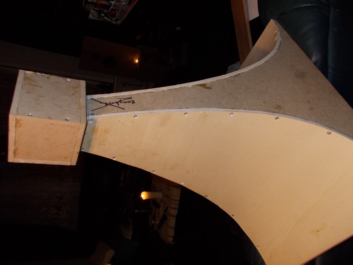
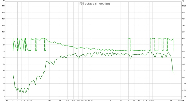
Here is what he has achieved so far with purely passive means - no EQ, no DSP, no PEQ, nothin' but a 6.8uF cap and elbow grease and a file. Remarkable for a single Visaton FR8.
More info here:
http://www.diyaudio.com/forums/full...ll-range-tractrix-synergy-53.html#post4464551
Here is what he has achieved so far with purely passive means - no EQ, no DSP, no PEQ, nothin' but a 6.8uF cap and elbow grease and a file. Remarkable for a single Visaton FR8.
More info here:
http://www.diyaudio.com/forums/full...ll-range-tractrix-synergy-53.html#post4464551
Last edited:
After doing some more research I agree. I also took the time to make sure I have a PML-solution that works, the increase in solution time is no doubt worth it as the sims are still reasonably fast (about 15 mins 1-20 kHz in 27 steps).You need to change the spacing by a significant amount which is normally a doubling or halving. The differences should show up at high frequencies not low frequencies. What is causing differences at low frequencies? Why are differences not being seen at high frequencies?
In a study like this you need to be able to see the what you are measuring. I would suggest running 2, 4, 8, 16, 32 elements per wavelength on a 2D grid and plotting something sensitive to numerical error. If the grid is created by subdivision then something that usually works well is to take the solution with the 32 elements per wavelength as a reference, evaluate the error norm for the other solutions with respect to the reference and plot on a log axis. The slope of the error reduction should follow the order of the numerical scheme. If it doesn't then some other error is swamping the discretisation error (or the numerical scheme is inconsistent which is unlikely for an established commercial code). That some other error is likely to be a incorrect or misbehaving boundary condition.
I have now removed the variation of geometry with frequency as this doesn't seem to be needed for the PML boundary condition. The BSC outlet apparently had more effect on the inlet.
As you said earlier I should make the convergence study for one frequency and a larger span of elements/wavelength. I've kept the frequency at 10^3.8 (6300 Hz) and the PML at 0.3 m and 6 layers (I'll do a study of this too later). The solution is considered "correct" at 16 elements/wavelength and I'm plotting the Norm of the difference in two points: One in the simulated volume and one in the far field.
Results
12 cm from membrane on axis
Linear:

Logarithmic:

2 m from membrane on axis (far field)
Linear:

Logarithmic:

Is this the correct approach? How do we chose an adequate amount of elements/wavelength from this information?
/Anton
Is this the correct approach? How do we chose an adequate amount of elements/wavelength from this information?
It is good to see the PML boundary condition is now working reasonably because simple exit conditions are usually only appropriate when placed a long way away from the working section where the waves are crossing the boundary close to 90 degrees.
You need to know the order of the elements you are using. For example, if they are 3rd order then when you double the grid the error should reduce by a factor of 2^3 = 8. If the error only reduces by, say, 4 then there is something wrong (e.g. a boundary condition evaluated at too lowly an order) even though the plot may look correct for a second order element. What is the order of the elements you are using given the way you are using them (some elements have a higher order on a uniform grid with the leading term in the truncation error cancelling).
The spacing needs to be on a log-scale as well in order for a correctly behaving scheme to asymptote to a straight line with the slope being the order of the scheme.
Normally one evaluates two types of error: the average throughout the solution and the worst point. This involves a calculation of the error for each element and a check to find the largest. Most codes will have functions that do this for you if you pass them the reference solution. Creating the reference solution on each grid level will require interpolation but, again, most codes have functions that perform the interpolation for you. For higher order FE schemes you need to interpolate using the shape functions of the elements if the nodes are not in exactly in the same location on each grid (achieved by subdivision). I am not familiar with the details of COMSOL but it is almost certain these functions will be provided somewhere.
Looking at the plots I would suggest dropping all but the 2, 4, 8, 16 and spending a few hours to get a 32 result because the second plot has clearly not settled at 16. What you should see is a wiggly plot when under resolved followed by an approach to a straight line with a slope following the order of the numerical scheme. The straight line should continue down to a noisy flat line at machine roundoff somewhere around 1.0e-14 for double precision but this will vary with how the errors are normalised.
The required number of elements per wavelength will follow from the order of the scheme and the form of the grid. Once the average error is "on" the straight line for the order of your scheme and the maximum error is not stuck at a high value but coming down in something like the same way then you can have some confidence that large systematic errors (i.e. invalid combinations of boundary condition) are not present in the solution.
Once you have a solution that is essentially the solution you would get with an infinitely fine grid plus some discretisation error then the question becomes how far do I need to reduce the discretisation error? This depends on how sensitive whatever you want from the solution is to discretisation error and how much you can back-out the effects of discretisation error that is present in the solution.
Your guidance is of great help, I'm very grateful!It is good to see the PML boundary condition is now working reasonably because simple exit conditions are usually only appropriate when placed a long way away from the working section where the waves are crossing the boundary close to 90 degrees.
You need to know the order of the elements you are using. For example, if they are 3rd order then when you double the grid the error should reduce by a factor of 2^3 = 8. If the error only reduces by, say, 4 then there is something wrong (e.g. a boundary condition evaluated at too lowly an order) even though the plot may look correct for a second order element. What is the order of the elements you are using given the way you are using them (some elements have a higher order on a uniform grid with the leading term in the truncation error cancelling).
The spacing needs to be on a log-scale as well in order for a correctly behaving scheme to asymptote to a straight line with the slope being the order of the scheme.
Normally one evaluates two types of error: the average throughout the solution and the worst point. This involves a calculation of the error for each element and a check to find the largest. Most codes will have functions that do this for you if you pass them the reference solution. Creating the reference solution on each grid level will require interpolation but, again, most codes have functions that perform the interpolation for you. For higher order FE schemes you need to interpolate using the shape functions of the elements if the nodes are not in exactly in the same location on each grid (achieved by subdivision). I am not familiar with the details of COMSOL but it is almost certain these functions will be provided somewhere.
Looking at the plots I would suggest dropping all but the 2, 4, 8, 16 and spending a few hours to get a 32 result because the second plot has clearly not settled at 16. What you should see is a wiggly plot when under resolved followed by an approach to a straight line with a slope following the order of the numerical scheme. The straight line should continue down to a noisy flat line at machine roundoff somewhere around 1.0e-14 for double precision but this will vary with how the errors are normalised.
The required number of elements per wavelength will follow from the order of the scheme and the form of the grid. Once the average error is "on" the straight line for the order of your scheme and the maximum error is not stuck at a high value but coming down in something like the same way then you can have some confidence that large systematic errors (i.e. invalid combinations of boundary condition) are not present in the solution.
Once you have a solution that is essentially the solution you would get with an infinitely fine grid plus some discretisation error then the question becomes how far do I need to reduce the discretisation error? This depends on how sensitive whatever you want from the solution is to discretisation error and how much you can back-out the effects of discretisation error that is present in the solution.
To answer your question: COMSOL uses a second order tetrahedral mesh, except in the PML where they are prisms (also second order). Here is what the mesh looks like for my latest sim:
2 elements/wavelength:

20 elements/wavelength:

I tried running the 32 elements/wavelength but ran out of memory (during LU factorization). I chose to try 20 elements/wavelength and got a solution. Only using 2, 4, 8 and 16 seems too coarse, I can't tell what happens between 8 and 16. So I added a few more, now it's 2, 4, 6, 8, 10, 12, 16. Solution time for these are: 1, s, 1 s, 4 s, 16 s, 25 s, 47 s, 3 min, 8 min (20 elements). I'm using the frequency 10^3.8 (~6300 Hz) as I noticed that the mesh stayed almost constant at low elements/wavelength when the frequency was low. This is caused by details in the geometry that has to be resolved anyhow.
The PML seems to work when the thickness is set to 0.3 m, but not if it is set to 0.1 m. There is some scaling going on (Rational coordinate stretching) that I'm not sure how to handle and it's probably the reason why.
There is also a setting for Relative tolerance, it is set to 0.001. Does that need to be altered?
I've assumed that I should set the start of the PML so that the waves hit them as perpendicularly as possible. This also reduces the domain volume substantially. Is that the correct approach?
Results
Estimated error using average SPL in the domain:

Estimated error using maximum SPL in the domain:

A second order element should then give 1/4 of the error if I double the elements/wavelength, correct? I added such a line to the last figure:

Somethings fishy.
This is what the SPL looks like (for 16 elements):

On average a few dB on the outer shell.
/Anton
That is a reasonable choice for a flexible general purpose element. However, unlike many other types of simulations, sound is smooth and requires an even grid distribution without regions of fine grid to resolve steep gradients. Higher order elements using hexahedrons can be expected to bring significant benefits in terms of increased accuracy/reduced computer costs. But if the standard approach is working well enough it may be prudent to stick with it.To answer your question: COMSOL uses a second order tetrahedral mesh, except in the PML where they are prisms (also second order).
The order in the PML doesn't matter since it's only task is to dissipate the sound without reflection anyway it can.
This seems to be showing flat triangular surfaces. If you are using second order elements they can (and probably should be) fitted to your curved geometry. The grid generator may or may not do this depending on how it works and/or is configured. The plot may not be representative of what is actually used in the simulation.Here is what the mesh looks like for my latest sim:
2 elements/wavelength:
Direct methods can only be used with relatively coarse to medium density grids. Fine grids require the use of iterative methods. There will be a setting somewhere to change the solver and some advice on appropriate methods and settings to use for acoustics problems. Iterative methods are more prone to failing to generate a solution than direct methods but you need to use them for fine grids.I tried running the 32 elements/wavelength but ran out of memory (during LU factorization).
The reference solution contains discretisation errors which are going to be significant for grids that are almost as fine (e.g. the 16 and 20). If the coarse grids do not subdivide everywhere then the discretisation error is not being raised uniformly everywhere and they represent the error on a mixture of grid levels. Both these will be influencing the results.I chose to try 20 elements/wavelength and got a solution. Only using 2, 4, 8 and 16 seems too coarse, I can't tell what happens between 8 and 16. So I added a few more, now it's 2, 4, 6, 8, 10, 12, 16. Solution time for these are: 1, s, 1 s, 4 s, 16 s, 25 s, 47 s, 3 min, 8 min (20 elements). I'm using the frequency 10^3.8 (~6300 Hz) as I noticed that the mesh stayed almost constant at low elements/wavelength when the frequency was low. This is caused by details in the geometry that has to be resolved anyhow.
I cannot help with the details of the particular PML implementation or what the grid represents. It is normal to need to read the manual for guidance about what parameters to fiddle with and then do a few tests.The PML seems to work when the thickness is set to 0.3 m, but not if it is set to 0.1 m. There is some scaling going on (Rational coordinate stretching) that I'm not sure how to handle and it's probably the reason why.
There is also a setting for Relative tolerance, it is set to 0.001. Does that need to be altered?
Maybe. A PML often wants the first element in the layer to be very close to the corresponding one outside the layer to help with the "perfect matching". In your case the elements are both of different shape and with a large difference in size. A PML is more tolerant of waves crossing at angles than simple exit conditions and it may sometimes be more beneficial that the grids match closely and the waves cross at greater angles than the waves are more normal and the grids more distorted. But guidance on this sort of thing for your particular PML implementation is likely to be more accurate coming from COMSOL and perhaps a bit of experimentation rather than me.I've assumed that I should set the start of the PML so that the waves hit them as perpendicularly as possible. This also reduces the domain volume substantially. Is that the correct approach?
Have you perhaps logged the pressure difference twice? (i.e. logged SPL rather than pressure difference?)Estimated error using average SPL in the domain:
Estimated error using maximum SPL in the domain:
A second order element should then give 1/4 of the error if I double the elements/wavelength, correct? I added such a line to the last figure:
Somethings fishy.
Is the element actually a second order element or will it behave more like a third on the uniform grids you are using on the finer grids?
The plots are distorted at the fine end by having levels of discretisation error close to that in the reference solution and at the coarse end by not coarsening everywhere. This is likely to make both ends better than they really are.
There may be something fishy in the refinement study itself but the results are not suggesting problems with the solution. It may or may not be worth further effort to bring this aspect of the study to a tidy conclusion.
This is a refinement study that is close to yours. Do things line up?
The streaks in the PML may indicate it is misbehaving to some extent.This is what the SPL looks like (for 16 elements):
On average a few dB on the outer shell.
This is one of the draw-backs of COMSOL. There are not a lot of element types to chose from.That is a reasonable choice for a flexible general purpose element. However, unlike many other types of simulations, sound is smooth and requires an even grid distribution without regions of fine grid to resolve steep gradients. Higher order elements using hexahedrons can be expected to bring significant benefits in terms of increased accuracy/reduced computer costs. But if the standard approach is working well enough it may be prudent to stick with it.
This seems to be showing flat triangular surfaces. If you are using second order elements they can (and probably should be) fitted to your curved geometry. The grid generator may or may not do this depending on how it works and/or is configured. The plot may not be representative of what is actually used in the simulation.
I'm quite certain that the plot of the mesh is not representative of what is used in the simulation. It probably shows the lines as straight (and surfaces as flat). This is what the 2-element mesh looks like:

And this is what the pressure distribution is for that mesh:

I'll try an iterative solver.Direct methods can only be used with relatively coarse to medium density grids. Fine grids require the use of iterative methods. There will be a setting somewhere to change the solver and some advice on appropriate methods and settings to use for acoustics problems. Iterative methods are more prone to failing to generate a solution than direct methods but you need to use them for fine grids.
Ah, of course.The reference solution contains discretisation errors which are going to be significant for grids that are almost as fine (e.g. the 16 and 20). If the coarse grids do not subdivide everywhere then the discretisation error is not being raised uniformly everywhere and they represent the error on a mixture of grid levels. Both these will be influencing the results.
I could do some experiments where the last element in the domain is the same type as the elements in the PML.Maybe. A PML often wants the first element in the layer to be very close to the corresponding one outside the layer to help with the "perfect matching". In your case the elements are both of different shape and with a large difference in size. A PML is more tolerant of waves crossing at angles than simple exit conditions and it may sometimes be more beneficial that the grids match closely and the waves cross at greater angles than the waves are more normal and the grids more distorted. But guidance on this sort of thing for your particular PML implementation is likely to be more accurate coming from COMSOL and perhaps a bit of experimentation rather than me.
I have indeed! Here they are with SPL (dB) on y-axis, not log10(SPL):Have you perhaps logged the pressure difference twice? (i.e. logged SPL rather than pressure difference?)
Average:

Zoom in on 8-20 elements/wavelength:

Maximum:

Zoom in on 8-20 elements/wavelength:

I used this as a starting point actually. Also the reason why I used the SBC instead of PML.This is a refinement study that is close to yours. Do things line up?
My thought as well. Could it be due to the fact that the lines in the PML mesh does not follow the wave path?The streaks in the PML may indicate it is misbehaving to some extent.
I tried tightening the tolerance to 0.00001, it had no visible effect that I could find.
/Anton
Lots of choice is not always a good thing because it can lead to more messing about and the use of inappropriate elements. What I was looking for was an element tuned up for acoustics: high order because of the smoothness, low dispersion but with significant damping of the highest resolved frequency.This is one of the draw-backs of COMSOL. There are not a lot of element types to chose from.
The downside of using low order elements is the need to use more of them to achieve a given level of accuracy but if your runs are only taking 10 minutes or so then there doesn't seem to be much of a problem there.
The walls look curved suggesting the grid generator has placed the non-corner nodes on something like your geometry (you want a "best fit" rather than on). I am a bit surprised the grid was shown with flat surfaces because how would you check how well the grid and geometry were aligned?I'm quite certain that the plot of the mesh is not representative of what is used in the simulation. It probably shows the lines as straight (and surfaces as flat). This is what the 2-element mesh looks like:
And this is what the pressure distribution is for that mesh:
The zoom is not helpful because we want to see the shape and trend which would be helped by plotting the spacings as well as the solution difference on a log axis. When unresolved the curve should wiggle but then smooth out as the solution moves towards being resolved. The drop from 8 to 16 is about 7 which might be about right given the uniform grid but we would need more points to be sure. Depending on the details of the element and how the leading discretisation error term behaves on a uniform grid you may see the solution error order rise to close to what it would be on a perfectly uniform grid.I have indeed! Here they are with SPL (dB) on y-axis, not log10(SPL):
Average:
Zoom in on 8-20 elements/wavelength:
Maximum:
Zoom in on 8-20 elements/wavelength:
Changing the grid spacing and number should affect the absorbing ability so long as the PML remains stable. The wiggles at the heavily absorbing end suggest it may not be fully stable. I don't know the details of the PML in COMSOL and this post suggests they may have had some issues in the past. COMSOL themselves are almost certainly the best source of information on what to prod and poke to get it working efficiently.My thought as well. Could it be due to the fact that the lines in the PML mesh does not follow the wave path?
I tried tightening the tolerance to 0.00001, it had no visible effect that I could find.
Here is a comparison for the 2-element case with Geometry (blue), Mesh (green) and Solution (Red).Lots of choice is not always a good thing because it can lead to more messing about and the use of inappropriate elements. What I was looking for was an element tuned up for acoustics: high order because of the smoothness, low dispersion but with significant damping of the highest resolved frequency.
The downside of using low order elements is the need to use more of them to achieve a given level of accuracy but if your runs are only taking 10 minutes or so then there doesn't seem to be much of a problem there.
The walls look curved suggesting the grid generator has placed the non-corner nodes on something like your geometry (you want a "best fit" rather than on). I am a bit surprised the grid was shown with flat surfaces because how would you check how well the grid and geometry were aligned?

The mesh plot is clearly simplified to only show straight lines between nodes. Why? I don't know.
I don't see why the zoom isn't helpful, how else are we to see where the error starts decreasing linearly? I am plotting both error (SPL) and elements/wavelength on a logarithmic axis.The zoom is not helpful because we want to see the shape and trend which would be helped by plotting the spacings as well as the solution difference on a log axis. When unresolved the curve should wiggle but then smooth out as the solution moves towards being resolved. The drop from 8 to 16 is about 7 which might be about right given the uniform grid but we would need more points to be sure. Depending on the details of the element and how the leading discretisation error term behaves on a uniform grid you may see the solution error order rise to close to what it would be on a perfectly uniform grid.
Here are the results from the iterative solution. It took 16 hours (!) in total (2 s, 14 s, 2 min, 1 min, 2 min, 3 min, 12 min, 15.7 hours). Clearly more unstable than the direct solver.
Average:

Zoom in on 8-16 elements/wavelength:

Maximum:

Zoom in on 8-16 elements/wavelength:

Looks linear from 8-16, but the error at 16 is suspiciously low. Does this indicate that some other error has taken over, maybe tolerances? I'm thinking about what you said "The straight line should continue down to a noisy flat line at machine roundoff somewhere around 1.0e-14 for double precision but this will vary with how the errors are normalised."
I have a "Relative tolerance" set to 0.001. And when I look at the error estimate for the pressure (which is the solved variable) I get 0.0007 at 16 elements/wavelength. Just below the Relative tolerance, coincidence?
COMSOL 3.4 was a long time ago (2007). As it is said in the link it was already fixed in 3.5, so I'm hoping it works as intended now 🙂Changing the grid spacing and number should affect the absorbing ability so long as the PML remains stable. The wiggles at the heavily absorbing end suggest it may not be fully stable. I don't know the details of the PML in COMSOL and this post suggests they may have had some issues in the past. COMSOL themselves are almost certainly the best source of information on what to prod and poke to get it working efficiently.
/Anton
Are you taking a difference in SPL values (i.e. a difference of logged values) or logging a difference between values of pressure. The latter is correct.I don't see why the zoom isn't helpful, how else are we to see where the error starts decreasing linearly? I am plotting both error (SPL) and elements/wavelength on a logarithmic axis.
Why have you repeated the solutions you already have? And, more importantly, why have you not got the same answer? Did you change the grid or boundary conditions? If not, my guess is the iterative solution has not been sufficiently converged.Here are the results from the iterative solution. It took 16 hours (!) in total (2 s, 14 s, 2 min, 1 min, 2 min, 3 min, 12 min, 15.7 hours). Clearly more unstable than the direct solver.
There are a range of iterative methods and each tends to have parameters that can be adjusted to accelerate convergence. Inevitably the fastest convergence tends to be found with values of the parameters close to those which give no convergence. The waves in acoustics problems can cause many iterative methods problems because small changes do not remain local in the way they do with stress and heat transfer but can propagate across the solution region. If you think you may need to use finer grids finding out how to get quicker convergence is likely to be the worth the effort.
If you continue refining the grid the numerical errors will get smaller and smaller until they reach the limit of what can be represented by a double precision number which is around 14 significant figures. You are not going to get anywhere near this limit with your 3D simulation but in 2D using higher order elements it can be reached to demonstrate a numerical method behaving correctly.Looks linear from 8-16, but the error at 16 is suspiciously low. Does this indicate that some other error has taken over, maybe tolerances? I'm thinking about what you said "The straight line should continue down to a noisy flat line at machine roundoff somewhere around 1.0e-14 for double precision but this will vary with how the errors are normalised."
I don't know what relative tolerance means in your context. Is it a stopping tolerance for convergence? If so, and a zero field or random field has a "relative tolerance" of about 1.0 then it looks like a value one might accept for some engineering work but not when the objective of the simulation is too evaluate small errors.I have a "Relative tolerance" set to 0.001. And when I look at the error estimate for the pressure (which is the solved variable) I get 0.0007 at 16 elements/wavelength. Just below the Relative tolerance, coincidence?
The error estimate is a measure of how well converged the solution is (i.e. the degree to which adding up the terms on the LHS of a row in your matrix problems equals the RHS). This is different to the discretisation error which we are trying to estimate by subtracting the solution on an unresolved grid from our best guess at the answer using the finest grid.
Alright, here is abs(p(32)-p(i))) using a logarithmic scale on both x- and y-axis:Are you taking a difference in SPL values (i.e. a difference of logged values) or logging a difference between values of pressure. The latter is correct.

And log10(abs(p(32)-p(i)))) on a linear scale on y-axis:

Is this how it should be done? Doesn't look very good though, does it? I'm redoing the sim with a much tighter Relative tolerance (1e-6).
I repeated as the solution time is so small for all solutions but the last one and it would take me more time to combine them when it's done. The errorWhy have you repeated the solutions you already have? And, more importantly, why have you not got the same answer? Did you change the grid or boundary conditions? If not, my guess is the iterative solution has not been sufficiently converged.
It seems like a stopping tolerance for convergence. I think it takes an estimated error and divides it with the solution value and if that is small enough it considers the solution converged.There are a range of iterative methods and each tends to have parameters that can be adjusted to accelerate convergence. Inevitably the fastest convergence tends to be found with values of the parameters close to those which give no convergence. The waves in acoustics problems can cause many iterative methods problems because small changes do not remain local in the way they do with stress and heat transfer but can propagate across the solution region. If you think you may need to use finer grids finding out how to get quicker convergence is likely to be the worth the effort.
If you continue refining the grid the numerical errors will get smaller and smaller until they reach the limit of what can be represented by a double precision number which is around 14 significant figures. You are not going to get anywhere near this limit with your 3D simulation but in 2D using higher order elements it can be reached to demonstrate a numerical method behaving correctly.
I don't know what relative tolerance means in your context. Is it a stopping tolerance for convergence? If so, and a zero field or random field has a "relative tolerance" of about 1.0 then it looks like a value one might accept for some engineering work but not when the objective of the simulation is too evaluate small errors.
Alright, I'll be clearer in naming of my figures.The error estimate is a measure of how well converged the solution is (i.e. the degree to which adding up the terms on the LHS of a row in your matrix problems equals the RHS). This is different to the discretisation error which we are trying to estimate by subtracting the solution on an unresolved grid from our best guess at the answer using the finest grid.
/Anton
Yes that now looks more like a typical plot. Normally the spacings would go 2, 4, 8, 16,... because the grid would be created by subdivision but your grid refinement is not as precise and even and that will make it a bit more wiggly.Alright, here is abs(p(32)-p(i))) using a logarithmic scale on both x- and y-axis:
Is this how it should be done?
It looks OK to me given the way the grid was generated. What do you think is poor about it? Perhaps more importantly it is not throwing up anything to be concerned about given we lack the full details of how the particular element is supposed to work. It would be nice to get another level but without getting the iterative method working more efficiently it is perhaps not worth the effort particularly if you do not think you need to use the iterative method for your highest frequency runs.Doesn't look very good though, does it?
What does "absolute tolerance" and "relative tolerance" mean in COMSOL speak? What solver are you using? How many iterations did it take in the previous run. What did the plot of residual errors look like? Etc... It is hard to give much practical advise without knowledge of this sort of thing. And it is hard to get those sort of details across in posts like this.I'm redoing the sim with a much tighter Relative tolerance (1e-6).
By their nature iterative solvers can restart from where they left off and so if you use the solution of the previous run as the initial conditions it will save you 15.7 hours of regenerating the same thing. It is also fairly common to drop the stopping tolerance by 10 or 100 and then have a look rather than going all in for a possibly unnecessarily large reduction in one go because you can simply continue the convergence if needed without penalty. Similarly when playing with the parameters to seek faster convergence one would keep a partially converged solution as a restart condition so that if a solution diverges or blows up it is not a case of back to square one.
- Home
- Loudspeakers
- Multi-Way
- 3D-printing