As a general rule, software and people in general speak of the accurate farfield measurement distance being a function of the distance between the measurement microphone and source and the nearest reflective surface. Others indicate that though this provides a reflection free window, true farfield cannot me measured unless the measurement microphone is at least 2 wavelengths away from the sound source of the lowest frequency of interest. This would put a damper in the accuracy of full range (that is, for the low frequency) ground plane measurements.
I was having trouble understanding the basic generalizations of a farfield distance so I posted over at Partsexpress and got a responses that pointed me in the right direction. I learned that estimates seem to come from the solution of the Rayleigh Integral.
I messed around with the far field question some more and have come up with what I believe to be a better understanding of this. I just did not feel right following cookbook estimates. I am attaching a spreadsheet for any other OCD types who really want to understand what they are getting when they measure far field. There is always some degree of error in this measurement.
To use this spreadsheet, you enter data in the yellow boxes only. Enter the highest frequency of interest and the radius of your driver in question (in cm). The ka is then calculated and a list of various ka's are then filled in below in column A. Column B then calculates the actual equivilent frequency that the data in the table is representing.
If you enter an allowable error pct, the table will highlight which distances and ka's (frequencies) are within your limits. The r/a mulitplier allows you to modify the r/a ratios to see more extended ratios. The actual measurement distance that the r/a ratio is representing is calculated above.
This allows you to see the error based upon the expectation that in the farfield there should be a loss of 6.02 dB for every doubling of distance. It is based upon the solution of the Rayleigh Integral.
I believe my calculations to be solid but if someone sees any error, feel free to jump in. I hope that this hopes some other poor obsessive soul.
Jay
Attachments
Hi,
An interesting endevour but can you give a little more explanation? The +% is an error of a point source gain vs. near field real circular source SPL?
This looks like something where a plot of SPL vs. distance (the form we normally see near field boundaries determined via) would be of great help.
David S.
The error is based upon the expectation that in the true farfield, we see a drop of 6.02 dB per doubling of measurement distance. In reality, according to the Integral, this does not really occur until infinity as this is the only place that a circular disc would appear as a point source. When we do farfield measurements, there is an innate error due to this. As we move further away, the error decreases.
I could plot the SpL drop at each of the points for a particular ka (like John K did in the Partsexpress bulletin board response where I posted the question originally) against the 6.02 dB expectation, but this is a numeric way of visualizing it. John has already presented a graph of this over at Partsexpress, as I mentioned. It is under a thread that I started there regarding the actual farfield measurement distance last week.
Jay
I think that the bottom line is that, as with everything else we do with our speakers, there is a benefit cost ratio to our choices. The further away we measure our speakers, the less the farfield error will be...but there is a point of diminishing returns as our window narrows and therefore the bottom of our frequency range rises. We have to choose the best point for us. It is likely that a few pct of error is not a major deal an octave or two over the anticipated crossover point, in my opinion. In fact, this is what we have all been living with (at least for low frequency drivers) for a while, perhaps without thinking about it (according to the math as I understand it).
Jay
Jay
Here is the forum link to where John K's graphic is:
The Real Farfield Measurement Distance - Techtalk Speaker Building, Audio, Video, and Electronics Customer Discussion Forum From Parts-Express.com
Jay
The Real Farfield Measurement Distance - Techtalk Speaker Building, Audio, Video, and Electronics Customer Discussion Forum From Parts-Express.com
Jay
It looks to me like John K's analysis shows the answer well in graphical form.
Techtalk Speaker Building, Audio, Video, and Electronics Customer Discussion Forum From Parts-Express.com - View Single Post - The Real Farfield Measurement Distance
If you are above r/a = 1 (or certainly by r/a = 4) then you are in the farfield and level is dropping by 6 dB per doubling of distance. R is distance from source and a is radius of source. 4 radiuses or 2 diameters distance is sufficient.
Now, a cabinet radiates from its edges, so that should be considered as part of its size if you want very high accuracy, although it is probably a minor factor. With multiway systems you also need to consider the distance required for the far field geometry to hold. That is, the distance where the path length differences between drivers is near enough to the far relationship.
Certainly, if you achieve twice the long dimension of the cabinet you have covered every factor.
David S.
Hi Guys
This may offer some additional grist for thought;
Best,
Tom Danley
http://community.klipsch.com/forums/storage/3/550738/FarFieldCriteriaLdspkrBalloonData.pdf
This may offer some additional grist for thought;
Best,
Tom Danley
http://community.klipsch.com/forums/storage/3/550738/FarFieldCriteriaLdspkrBalloonData.pdf
Dave, I think that the point of my doing the math (which is pretty much in agreement with John's graph) is to look at the actual error that exists. Of note, I ran this by John prior to posting it though I can't vouch that he looked at it in detail).
I think that there is some confusion regarding farfield. In fact, when I have looked at modeling papers, the Rayleigh integral is felt to be inferior in it's model of farfield to BEM modeling, particularly at higher frequencies.
The most current AES measurements standards state that "this implies that the measurement distance from the acoustic center of the device
must be large with respect to: (1) the largest dimension of the radiator, and (2) the square of the largest
dimension of the radiator divided by the wavelength of the highest measurement frequency."
If one was to use an enclosure that was .6 meters tall and .2 meters wide, the longest dimension (the diagonal) would be .63 meters. Using the 2nd criteria, if you measure to 20,000 Hz, this would be .63^2*20000/344 or 23 meters. This made no sense to me. Even using half of this dimension, assuming the driver is centered on the baffle, it would be 5.76 meters to FF. Using just the driver, itself, let's say a 1 inch tweeter, the calculation would be .0254^2*20000/344 or 37.5 cm.
Looking at the table that I set up, at 38 cm, you could measure to 20Khz with .2% error. If you use the 63 cm size (of the enclosure diameter), at 20kHz, there is an 8.8% error at 23 meters.
John's graphic seems to be more in line with the use of just the driver. It also suggests that what we are using for our definition is also more along the lines of the driver. The enclosure provides a reinforcement of the sound signal starting with a frequency equal to the longest distance of the driver to the edge of the enclosure and ending with a freq equal to the driver distance to the shortest part of the enclosure. The distribution is based upon enclosure shape, reflectivity, etc.
Your suggestion of using twice the largest baffle dimension is likely to always put you in farfield by my calculations, but it is another rule of thumb that I was trying to get away from. I was trying to understand the why. As I mentioned before, the Rayleigh integral is not exact, but it at least provides an understanding of the cost/benefit ratio of a measurement distance along with one's window length calculation.
This is an educational endeavor for me and if you have more insights, I am not attempting to be argumentative here.
Jay
I am aware of the HF stretching of the far field transition distance and included it in my paper on line array modeling.
http://www.diyaudio.com/forums/mult...th-transducers-line-arrays-6.html#post2257395
Look at the 3rd PDF and you will see some graphs of a long multi-element array that, at 10kH, didn't settle down until past 15 times the array length. The periodic wobble of level comes from the rotating phase contribution of the outter elements. Once the end elements come mostly in phase with the center the response settles and you are in the far field. This, of course, is only true for the particular example of a multi-element line array, although this could be considered the sampled version of a continuous array.
I'm not totally sure how this reconciles with John's graphs that show the transition point to be essentially independent of frequency (the curve shapes below that are certainly different, but the transition frequency is not).
In the practical case all we care about is what distance gets us to the point where our curve, to a sufficient accuracy, agrees with the curve at infinity. For most speakers our source gets smaller at HF (multiway speakers, right?) and just worrying about the longest dimension seems to be a practical step.
David S.
Thank you for the very interesting links, Dave. I don't believe that we are in disagreement. I think that the only questions that arise are which radius to use for the spreadsheet and, at least for line arrays, your PDF suggests it is more of a longest dimension for line arrays. For individual drivers, it may be different, but this is good ground for a practical experiment.
Some time back, I measured a loudspeaker (2 driver with xover in place) at steadily increasing distances and watched as the high frequency did not appear to reach equilibrium until further back while the lower frequency driver showed a more rapid equilibrium (not quite the right word but it gets the point across). This would also be consistent with your PDF as the higher frequency reproduction would otherwise not really require longer measurement distances unless the baffle, and not the driver size, were being considered.
Putting this all together (both your work and mine as well as the balloon paper referenced by Tom), I think that the spreadsheet is a useful tool (biased as I might be) in helping to understand the approximate error in measurement for measurements taken at different distances and frequencies for different drivers. Indeed, using the spreadsheet, indicates that at 10kHz, for a 1 inch tweeter on a .2 meter wide baffle that is 1 meter tall and centered and 1/4 of the way from the top (longest dimension: 0.76m), you would still have a better than 3% error at 30 meters.
It seems to me that we are living with errored measurement but I have a tough time believing that we are living with so much error; I wonder if the baffle does not contribute to the response as much as the mobile portion of the diaphragm and therefore the use of the longest dimension might not be an accurate way of doing this?
Jay
Is that 3% in pressure? That would be about 1/4 dB. I would suggest you expand your spreadsheet to include dB conversion of results and even go to a more standardized presentation of graphed dB vs. drawaway distance. That is the best way to view it
As I looked at John's graphs a bit more it is clear that, below a certain frequency, all the nearfield curves merge. The nearfield effect is strong but independent of frequency. It is only higher frequencies where frequency becomes a factor at all. This is where the generalized frequency independent notion come from. At low frequencies,nothing matters but size. At high frequencies the circular unit must be considered as anular rings of potentially different phase (like my multiple point sources) and until you are far enough away for all rings to be in phase you will see a lower nearfield condition.
Still, if we cross from a large source to a small one at HF we are taking a large step in keeping the nearfield effects of HF nullified. The end result is that a typical system is still well represented at a distance of 2 or 3 diagonals away (line arrays excepted).
David S.
I would like to point out that the Rayleigh model for a circular disk is itself a simplification that does not match reality so be careful applying it to this situation.
In a fully accurate model of sound radiation from a finite source the far field is reached when the sound radiation modes approximate their far field assymtotic expressions. This differs for every mode which is what makes this transition frequency dependent in the non-modal case. Now the far field expression is what we want, but that does not mean that we cannot get the far-field equivalent from near-field data. We simply have to find the near-field expressions and then use those to calculate what the far-field would be. Depending on how you view the problem this can be relatively straightforward or impossible. With a flat disk in an infinite baffle it is basically impossible if the Reyleigh integral approach is used (although the concepts can be extended along the lines I will outline below and then this farfield adjustment can be made. This was recently done in an AES article).
The transition from near field to far field is simple when one has a modal representation of the sound radiation. That is because the modal radiation has precsiely know modal functions which are defined for all space and hence transitions from one location to another are easy. But how does one get the sound radiation as a set of radiation modes? The sound field - at any distance - can be expanding into its modes using principles of orthogonality just as in any other modal representation (the modes are orthogonal). This expansion results in an equivalent set of source velocity modes that would have to have occured on some surface - usually defined to be close to the real surface of the source (but this is not a requirment). For what I do these modes are the spherical ones since my sources are in free space (on a high platform).
This is not really so hard to understand because there are some cases that are quite simple. For example, a line array. In a line array the polar sound radiation (in the plane of the line) is simply the Fourier transform of the source velocity distribution. Thus measureing the field anywhere in this plane allows one to calculate the source velocities from the known measurement distance (usually an arc of constant radius) and from these known velocities on could find what the far-field radiation would be, or actually anywhere in between - including right at the source, i.e. source recontruction from sound radiation measurements. This later etechnique is often called Nearfield Acoustic Holography or "Fourier Acoustics" per Earl Williams book.
For a square source in an infinite baffle we would use a two dimensional Fourier transform. For a circular source in a flat baffle the well known Bessel transform is used (well known because this is the transform used for lenses in optics or radar when circular aperature are used - see the classic text "Introduction to Fourier Optics" by Goodman).
For me I use Spherical Harmonics -Lengendre functions and Spherical Bessel Functions. I measure at say 1 or 2 meters, find the equivalent source modes and then recalculate what the sound field would be at say 10 meters. Whala! No need to wory about nearfield or far field effects with one exception. A different approach has to be used when one falls below the fequency of the window because the data is contaminated by this truncation. Handle that and you have a completly valid far-field measurement done in a small room. There is also an issue of stability of the reconstruction at LFs and when one gets too close. The numerics can get unstable and this has to trapped or the calculations fail. This is never a problem that is not obvious - all of a sudden the modes just go off to infinity. This is because for high order modes at low frequencies the radition is so small that noise in the data can make it appear that a very large contribution must have been necessary, i.e. singular behavior.
I have been using this technique for years, but it took me almost five years to get working correctly. I have thought about writting all this up, and I'd like to do a book called "Modal Sound Radiation" because these techniques are so powerful, but it all takes time.
Last edited:
That is 3% error based upon the expectation of 20*Log(2) drop in dB level so it would be 3% of 6.02 dB or .18 dB.
The spreadsheet actually calculates a relative dB level and calculates the error. I originally had the dB drop also on there but I then hid it to make it more simple.
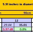
In the attachment, you can see that I included one block for a 7.5 cm radius speaker at 90 cm where the relative drop is a 5.97 dB drop (29.04 to 35.01 dB). This, when compared to 20*LOG(2) is a 0.8% error.
It would certainly be no trouble to reformat what is visible to demonstrate dB instead of pct if folks feel this would be more valuable to them.
Jay
The spreadsheet actually calculates a relative dB level and calculates the error. I originally had the dB drop also on there but I then hid it to make it more simple.
In the attachment, you can see that I included one block for a 7.5 cm radius speaker at 90 cm where the relative drop is a 5.97 dB drop (29.04 to 35.01 dB). This, when compared to 20*LOG(2) is a 0.8% error.
It would certainly be no trouble to reformat what is visible to demonstrate dB instead of pct if folks feel this would be more valuable to them.
Jay
Attachments
I see. It is % error of the dB vs expected dB for that step. It is a per step rather than cumulative error.
You would still be better served by showing total dB deviation relative to a point source with the same far field pressure. (as per John's graphs, the various curves can be directly compared to the 6dB per distance-doubling asymptote. It shows what you want to know: "what is my level vs. distance and where does it deviate from the ideal as I get closer to the source".
I can also look at John's graphs and see where the error hits 1dB or 3dB, which is what I really want to know.
David S.
It seems to me that we are living with errored measurement but I have a tough time believing that we are living with so much error; I wonder if the baffle does not contribute to the response as much as the mobile portion of the diaphragm and therefore the use of the longest dimension might not be an accurate way of doing this?
Jay
Sure, the direct component from the driver is primary and most people are happy to consider near field effects by considering driver size alone.
There are some useful diffraction modeling programs available (the Edge, etc.) and for frequencies where diffraction related response is minimal, using the cabinet dimensions is "overkill".
I guess the answer depends on how you are asking the question:
1) at what distance am I absolutely in the far field? (consider the longest dimension)
2) at what distance am I clearly in the near field? (consider the driver dimension)
David
I'm not totally sure how this reconciles with John's graphs that show the transition point to be essentially independent of frequency (the curve shapes below that are certainly different, but the transition frequency is not).
If you plot up additional curves for increasing ka, you will see that in fact the transition point is dependent on frequency and in line with the second formula given in the AES measurements standards: “(2) the square of the largest dimension of the radiator divided by the wavelength of the highest measurement frequency."
As an example I attached a table with calculations for a 12” diameter piston. You can see the calculated transition distances for each ka value correspond well with where the curves merge in with the -6dB slope. A derivation of this far field break-point formula can be found in the AES paper "The Acoustic Radiation of Line Sources of Finite Length" by Lipshitz & Vanderkooy.
AES E-Library The Acoustic Radiation of Line Sources of Finite Length
I’m not sure how relevant this calculated far field transition point is for a 12” woofer which probably won’t be crossed over above 1kHz and most likely wouldn’t be radiating uniformly out to the cone edges. But for line sources made up of small drivers, or large area radiators like ESLs it is a good guideline. When designing ESLs, you often have to take into account that typical listening distances will place the listener in the far field relative to the width, but near field relative to the height.
Attachments
Last edited:
For me I use Spherical Harmonics -Lengendre functions and Spherical Bessel Functions. I measure at say 1 or 2 meters, find the equivalent source modes and then recalculate what the sound field would be at say 10 meters. Whala!
When recalculating the sound field at 10 meters for say a 12” pulp cone woofer, is the cone assumed to be perfectly rigid?
Or can you include the behavior of the woofer cone as far as shrinking of source size.
Dave, it is a cumulative error. You do not see that it is being compared to a half distance as this portion of the calculation is not visible.
Earl, thanks for jumping in. Is there any way to calculate this out using your method in such a way that anyone would be able to identify a relative error at different points with different drivers? If not, is my approach within a reasonable error range? If not, any suggestions as to how I might make it so?
bolserst, as you pointed out, the curves do asymptote but not quite as early as it appears on John's graph. Where the curve joins the asymptote appears to be frequency based.
Jay
When recalculating the sound field at 10 meters for say a 12” pulp cone woofer, is the cone assumed to be perfectly rigid?
Or can you include the behavior of the woofer cone as far as shrinking of source size.
Since we are talking about measurements of real speakers then it doesn't matter what that speaker does, it will be accounted for as long as the number of terms in the expansion is sufficient to cover it. From what I have done, I see no differences in the data beyond about 16 terms up to about 10 kHz.
- Status
- This old topic is closed. If you want to reopen this topic, contact a moderator using the "Report Post" button.
- Home
- Loudspeakers
- Multi-Way
- The Real Farfield Distance