Nothing wrong with you measurement, but as you put it, it is a burst which is a transient signal. It takes time for the system to respond to it, and take sime for the system to stop after the signal is removed. How long depends on the form of the impulse and test frequency.
It is not the measurements which are flawed, but your logic.
Sure a sine burst is a transient signal !
But - for the purpose used, I'd say it's absolutely suitable.
Compare the simus and the measurements > perfect correlation to theory.
Where do you see my logic flawed ?
If we clearly see the amplitude of a given frequency varying with time, the most simple conclusion is to state: "there is different FR depending on the time we look at".
Michael
Last edited:
Where do you see my logic flawed ?
If we clearly see the amplitude of a given frequency varying with time, the most simple conclusion is to state: "there is different FR depending on the time we look at".
Consider a single, ideal, high Q resonator---a tuning fork, for example. If you drive such a resonator with an on-resonance sine wave whose amplitude is constant (after the initial onset), the amplitude of the tuning fork's oscillations will increase over time as it approaches a steady state. It takes awhile for the oscillations to build up to their final amplitude even though the driving force isn't varying with time. In this case the "amplitude of a given frequency [varies] with time." Nonetheless, the amplitude portion of the frequency response consists of a single narrow peak. You don't need a different frequency response for each instant in time to convey the fact that the fork may resonate with different amplitudes at different times.
In other words, once you know the frequency response (magnitude and phase) you have all you need to predict the observed time varying response of the tuning fork. You can always play with different time windows and ask how much each frequency appears within a particular period of time, but that doesn't change the fact that a if you know the magnitude and phase response as a function of frequency you have all you need to predict the fork's response in the time domain.
Varying the time windows and recomputing the Fourier transform, as is done to create a CSD plot, is just a way to view the information differently. It doesn't add any new information. Everything in a CSD plot is fully contained in an impulse response plot (amplitude vs. time) or in the corresponding time-invariant frequency response plot (magnitude and phase versus frequency).
Bottom line: Variation of amplitude over time does not imply variation in the frequency response over time.
Few
I was really scratching my head about this wiggle of the TD15M. Looked up half a dozen responses of 12" & 15" drivers at Brandon's Driver Measurements - drivervault and all had that same thing more or less.
I think it is a delayed damped back-bounce from the shockwave through the type of spider used for that sort of pro drivers, isn't it? Or is that too simple?

I was wondering the same thing - a transverse wave in the spider. This would explain the reversal, since a transverse wave is reflected inverted. It would also explain why ALL of the AE 15" speakers exhibit this response. I wonder if they all use the same spider?
The time/distance equation would therefore depend on the propagation speed of the transverse wave in the spider, and NOT on the speed of sound in air.
Thoughts?
As per rules of the forum, personal messages are ment to be kept personal....
You'll gonna keep that 10 words as a secret ??
Michael

As per rules of the forum, personal messages are ment to be kept personal.
Ok - so I'll be patient until those ten words got brought down the hill - carved into two stone plates...

Micheal
Consider a single, ideal, high Q resonator---a tuning fork, for example.
Few

Bottom line: Variation of amplitude over time does not imply variation in the frequency response over time.
Few
Possibly true, but not necessarily the other way around.
Look at:
- the blue trace = resonant behaviour
- and the red trace = CMP behaviour
to see what I mean
With resonant behaviour (blue trace) we have the built up and after source signal (green trace) stops, there is decay.
With CMP behaviour (red trace) we have change of frequency response after delay time and - after source signal stops - a tail the length of exactly the original delay - which is *not* decaying.
Michael
Last edited:

Do you know where you are going to place the ribbon tweeter or are you going to try it first without one??
I'll go without tweeters at first, and work on getting the crossover dialed in. I expect to keep the TD15M and Azurahorn as close together as possible, which means the tweeter will have to stay out of the way. A few possibilities:
1. Above the Azurahorns, time-aligned of course. Hard to imagine an attractive way of doing this.
2. Next to the Azurahorns, atop the TD15M cabinets.
3. Facing rearward, as Hiraga has done with his highly-regarded JH-MS15 Reference speakers. (Link: 6moons industry features: Jean Hiraga)
I would like to experiment with these placements before designing permanent mounting provisions.
Gary Dahl
Bottom line: Variation of amplitude over time does not imply variation in the frequency response over time.
If the amplitude of the signal at a given frequency differs with time, the "frequency response" differs identically. I measure the frequency response of a system and it is flat. Then I measure it again some time later and there is now a sharp resonant peak. It just means the resonance took time to build up (implying high Q).
I wonder if you might have intended to say,
"Variation of amplitude over time does not imply variation in the resonant frequency over time."
The variation in amplitude is a signal. It appears in the form of new frequencies. For example, a 1 KHz sine wave varying sinusoidally in amplitude at 100 Hz. When analysed in the frequency domain, it appears as a constant amplitude 1 Khz signal and two new signals, 0.9 KHz and 1.1 KHz.
Likewise, analysing the spectrum of a resonance building up due to excitation will show "sidebands" at frequencies related to the time constants (Q) of the resonance.
Hi Don,
No, I actually meant what I posted. The system (speaker, for example) has a frequency response. It doesn't have different frequency responses depending on which signal it's fed or on when you happen to measure them.
The frequency response can be expressed in the frequency domain as a magnitude and phase response as a function of frequency or as real and imaginary parts as a function of frequency. The system's response can also be characterized in the time domain by an impulse response (amplitude as a function of time). Any of these depictions are different ways of expressing the same information. If you have one, you have everything you need to produce the others.
Perhaps the confusion lies here: "Frequency response" and "function describing how much each frequency contributes to a given output signal within a particular time window" are not the same thing. To the extent that it's linear and time invariant, a system is uniquely characterized by its frequency response or, equivalently, by its impulse response (ignoring directivity issues). Given one of those, you have everything you need to compute what the system's response will be at any time to any input signal.
This is not the same as saying the system produces the same amount of sound at each frequency within each time interval no matter what signal it's fed. It's pretty clear all components in an audio system can produce different amounts of each frequency in different time intervals, otherwise they couldn't reproduce music.
I hope I'm not just muddying the waters with this post. I really think it comes down to the accepted definition of the frequency response of a system. This site is hardly authoritative, but perhaps it'll explain things more clearly than I have.
Few
I wonder if you might have intended to say,
"Variation of amplitude over time does not imply variation in the resonant frequency over time."
No, I actually meant what I posted. The system (speaker, for example) has a frequency response. It doesn't have different frequency responses depending on which signal it's fed or on when you happen to measure them.
The frequency response can be expressed in the frequency domain as a magnitude and phase response as a function of frequency or as real and imaginary parts as a function of frequency. The system's response can also be characterized in the time domain by an impulse response (amplitude as a function of time). Any of these depictions are different ways of expressing the same information. If you have one, you have everything you need to produce the others.
Perhaps the confusion lies here: "Frequency response" and "function describing how much each frequency contributes to a given output signal within a particular time window" are not the same thing. To the extent that it's linear and time invariant, a system is uniquely characterized by its frequency response or, equivalently, by its impulse response (ignoring directivity issues). Given one of those, you have everything you need to compute what the system's response will be at any time to any input signal.
This is not the same as saying the system produces the same amount of sound at each frequency within each time interval no matter what signal it's fed. It's pretty clear all components in an audio system can produce different amounts of each frequency in different time intervals, otherwise they couldn't reproduce music.
I think this may reflect a confusion between a frequency response and a snapshot of the spectrum of a system's response to some signal over some particular time interval. The former does not vary with time, and the latter definitely does. The display of a real time spectrum analyzer changes over time because it's showing how much each frequency contributes to the signal over some time period. It's varying primarily because the input signal is varying, and also because the response of a system with a given frequency response takes time to approach a steady state when it's driven by a signal. It's not varying because the system's frequency response has any time dependence.If the amplitude of the signal at a given frequency differs with time, the "frequency response" differs identically.
I hope I'm not just muddying the waters with this post. I really think it comes down to the accepted definition of the frequency response of a system. This site is hardly authoritative, but perhaps it'll explain things more clearly than I have.
Few
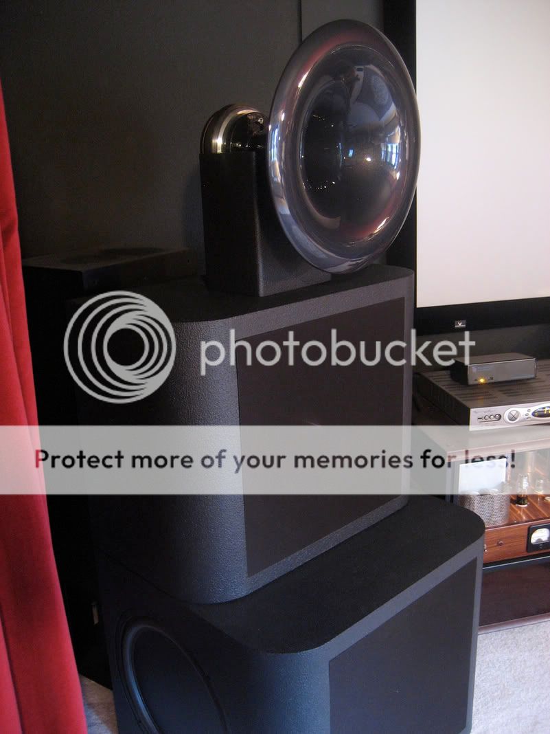
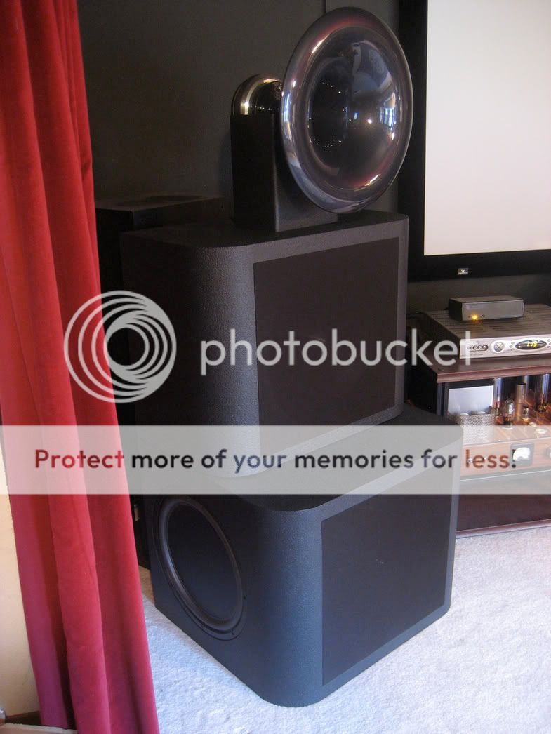
Picture time!


Okay, what exactly are we looking at here? What drivers were settled on and what are the loading configurations and the crossover points? I'd like to see a full system design description. I'm asking because I really haven't been following this thread much since it went over 3000 posts. I'm glad to see something actually got built.
Hi Don,
No, I actually meant what I posted. The system (speaker, for example) has a frequency response. It doesn't have different frequency responses depending on which signal it's fed or on when you happen to measure them.
(...)
... It's varying primarily because the input signal is varying, and also because the response of a system with a given frequency response takes time to approach a steady state when it's driven by a signal. It's not varying because the system's frequency response has any time dependence.
... but if "the response of a system with a given frequency response takes time to approach a steady state when it's driven by a signal", then its frequency response has time dependence. But I see what you mean, and I think we're in agreement:
... I really think it comes down to the accepted definition of the frequency response of a system. ...
I originally wrote the same phrase in my post but edited it out before posting.
Thanks for the book pointer.
Okay, what exactly are we looking at here? What drivers were settled on and what are the loading configurations and the crossover points? I'd like to see a full system design description. I'm asking because I really haven't been following this thread much since it went over 3000 posts. I'm glad to see something actually got built.
Description was in post 6595:
When the speakers are complete, each channel will consist of the following components:
Aurum Cantus G-3 ribbon (above ~8 kHz).
Azurahorn AH-425 with Radian 745PB driver (900 Hz to ~10 kHz).
AE TD15M in 3 cu ft sealed enclosure (75 Hz to 900 Hz). LF rolls off naturally.
AE TD15H and two PR15-700 passive radiators in 5 cu ft enclosure, actively powered. This will be allowed to overlap with the sealed cabinet in order to fill in below the baffle step, about 200 Hz.
The enclosures for both of the AE drivers are about 20" tall and 25" wide. The front vertical edges have a 4" radius. The lower (TD15H/PR15) cabinet depth is about 22", while the sealed (TD15M) cabinet is about 14" deep. The two cabinets will be stacked for a total height of about 40", and the Azurahorn and ribbon will be mounted on top. Definitely not a minimonitor!
At this point, all of the drivers are on hand, and all of the baltic birch and MDF parts have been cut. Today the first of the TD15M cabinets went through its first stage of glue-up. Assembly of remaining cabinets will continue through the coming week.
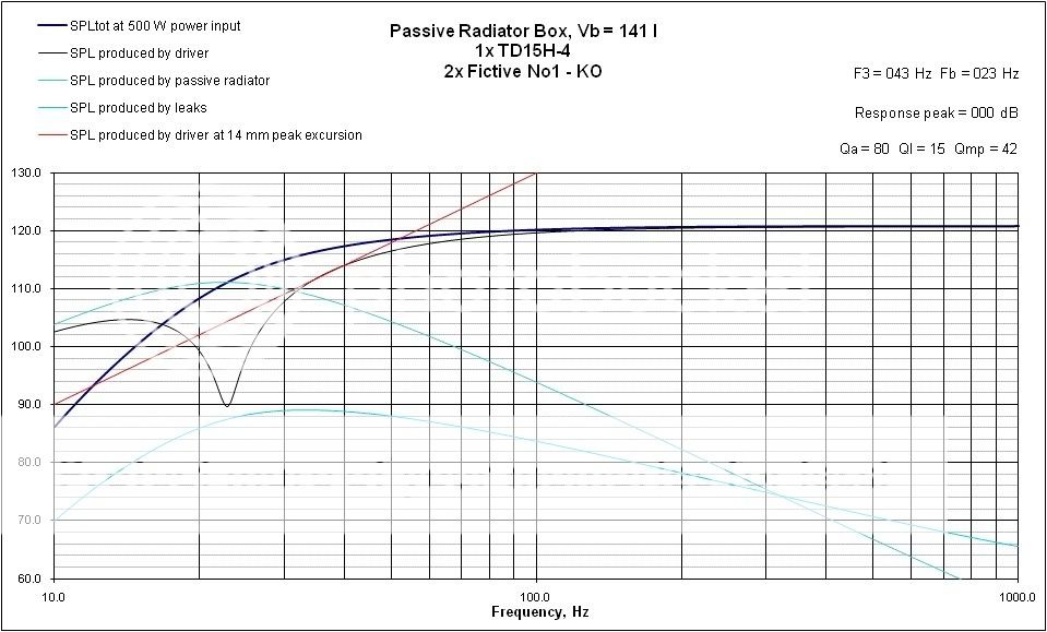
I chose the dual-woofer configuration because I wanted to have the ability to dial in the bass response shape. The TD15M is known for its excellent midrange, and I really liked the way the Unibox sims look for the the TD15H in the dual PR cabinet. Separate active power for the TD15H will allow me to adjust the lows for best in-room performance.
Here's a Unibox simulation of the TD15H-4 in the passive radiator enclosure:
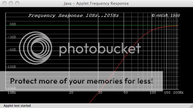
Here's a simulation of the TD15M-8A from the MH-Audio sealed-box calculator:
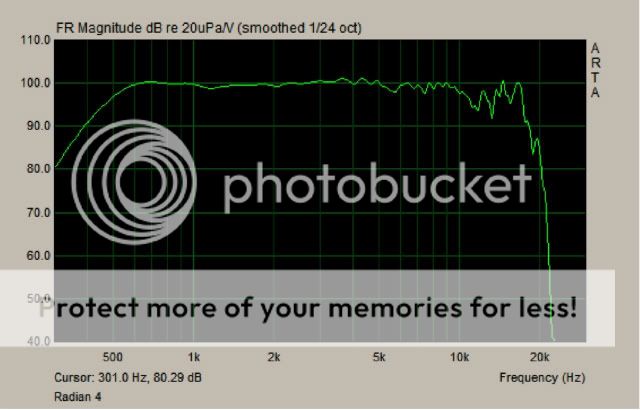
Here's the measured response of the Radian 745 in the Azurahorn:
Crossover development will commence this weekend, so these speakers haven't yet sung their first song.
Gary Dahl
I hope I'm not just muddying the waters with this post. I really think it comes down to the accepted definition of the frequency response of a system.
Few
Definitely you are not mudding the waters – quite in contrary – I'm actually happy you pointed out LTI such clearly, as I possibly wasn't so clear some times myself.
The question here is *if* we should look at CMP systems as to be LTI or not.
Seen as a whole – meaning from time zero to eternity, a CMP system definitely *is* both : time invariant and linear (and hence *can* be accessed for 100% correction in theory) - though I guess, the term „time invariant“ could also be interpretated differnently here. For sure a CMP system is „time invariant“ for each of the three time spans :
zero to delay time
delay time to end of input
end of input to end of input plus delay time
But however the math is defined – the net result with CMP is that FR varies with time we look at.
I could also state it different :
Looking only at a time window of „zero to delay time“ we *never* would get a clue that notches and bumps are happening in FR (which is not the case for „true“ LTI systems when we shorten the time window).
Also – conventionally EQ'ing out a „peak“ or „notch“ in FR of a CMP system will actually make performance in time domain worse (which also is not the case for „true“ LTI systems).
So we just as well could state that the concept of FR - meaning any FR plot actually - is quite useless (within the limits outlined) when it comes to CMP behaviour – but as a compromise its maybe more intuitively to speak of „FR changing in time“.
Michael
Last edited:
Seen as a whole – meaning from time zero to eternity, a CMP system definitely *is* both : time invariant and linear (and hence *can* be accessed for 100% correction in theory) - though I guess, the term „time invariant“ could also be interpretated differnently here. For sure a CMP system is „time invariant“ for each of the three time spans :
zero to delay time
delay time to end of input
end of input to end of input plus delay time
I should have added thats what appears to me as the "words meaning" of "LTI" and "time invariant" in the sense of "determined" (its definitely not me whose the math magician here).
Michael
- Home
- Loudspeakers
- Multi-Way
- Beyond the Ariel